REVISION DATE: 05-Apr-2018 12:48:20
The Heilum wave cal data.
Below are my graphs of the helium 100ms data. The file contains 20 images of the helium lamp source. All the data are dark subtracted. See each graph below for more detail.
Track Wavelength fits:
P(1,:) = [8.901595e-12 -2.402813e-08  3.258765e-05     0.3333437      351.2181]
P(2,:) = [9.881892e-12 -2.572831e-08  3.331966e-05     0.3334199      351.1705]
P(3,:) = [1.047805e-11  -2.75175e-08  3.512084e-05     0.3326449      351.3226]
P(4,:) = [1.037262e-11 -2.720671e-08  3.486411e-05     0.3326811      351.3602]
P(5,:) = [8.438948e-12 -2.338033e-08   3.23311e-05     0.3333294       351.298]
P(6,:) = [7.896375e-12 -2.238685e-08   3.17078e-05     0.3335079      351.2665]
P(7,:) = [7.617059e-12 -2.189509e-08  3.144473e-05      0.333548      351.2708]
P(8,:) = [5.337947e-12 -1.725272e-08  2.826917e-05     0.3343903      351.1881]
P(9,:) = [7.199289e-12  -2.12818e-08  3.122794e-05     0.3335913      351.2151]
P(10,:) = [4.996457e-12 -1.624577e-08  2.717494e-05     0.3349132      351.0612]
P(11,:) = [8.2102e-12 -2.314958e-08  3.222809e-05     0.3335027       351.147]
P(12,:) = [6.741428e-12 -2.013091e-08  3.013369e-05     0.3341071      351.0444]
P(13,:) = [6.204044e-12 -1.901195e-08  2.946179e-05     0.3342861      350.9646]
P(14,:) = [8.29303e-12 -2.318642e-08  3.220681e-05     0.3336872      350.9199]
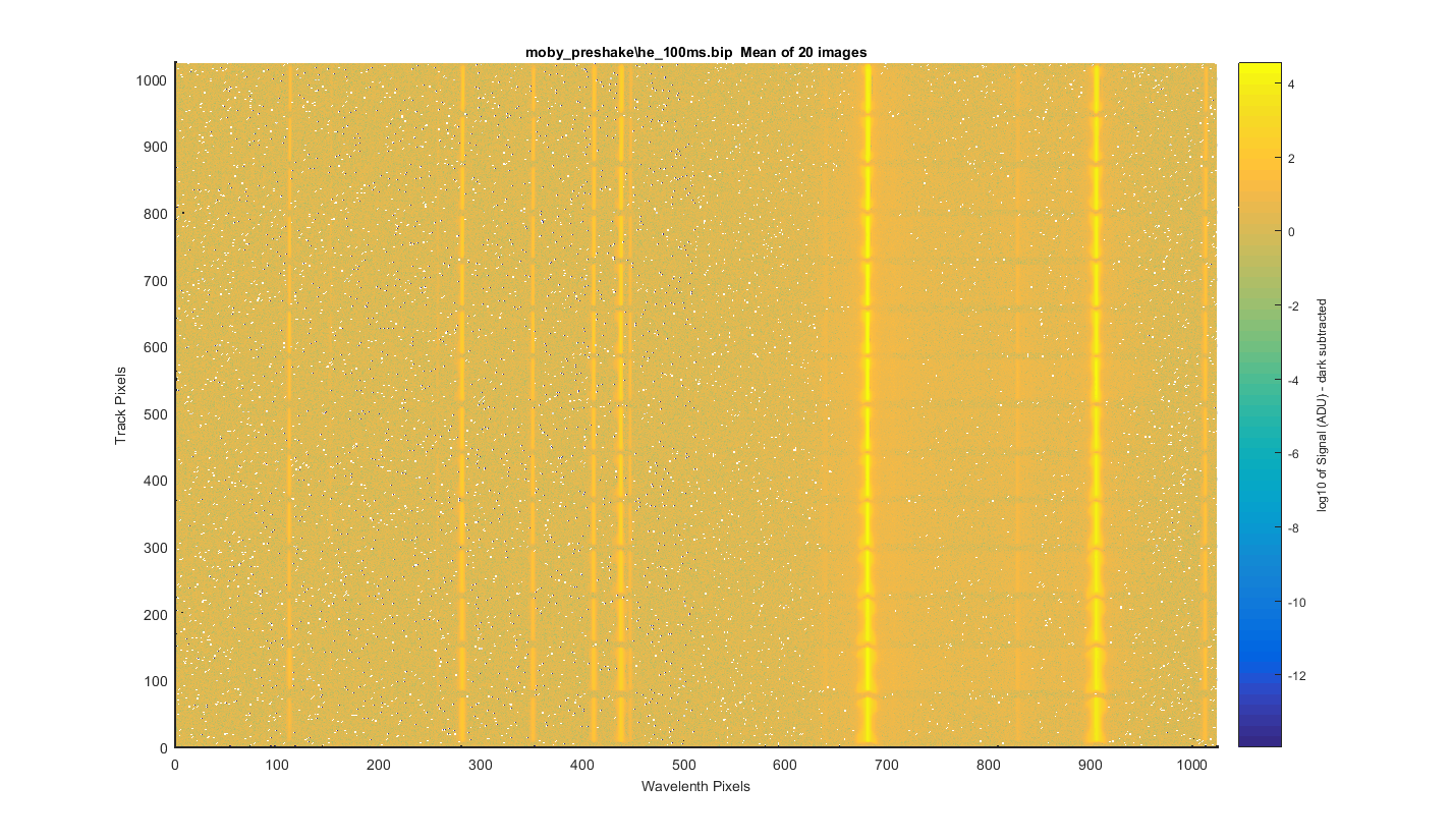
Figure 1
Resonon took dark scans for the two int times taken. So I meaned all the dark images for the 100ms data and subtracted it from the data before processing. I Then took the 20 images and meaned them to get the surface plot below.
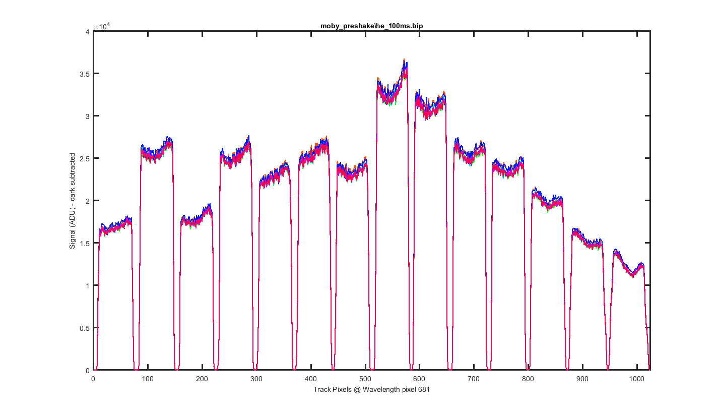
Figure 2
This is a cross section through the tracks at wavelength pixel 705, with one line for each of the 20 images. The tracks and their shapes look really stable.
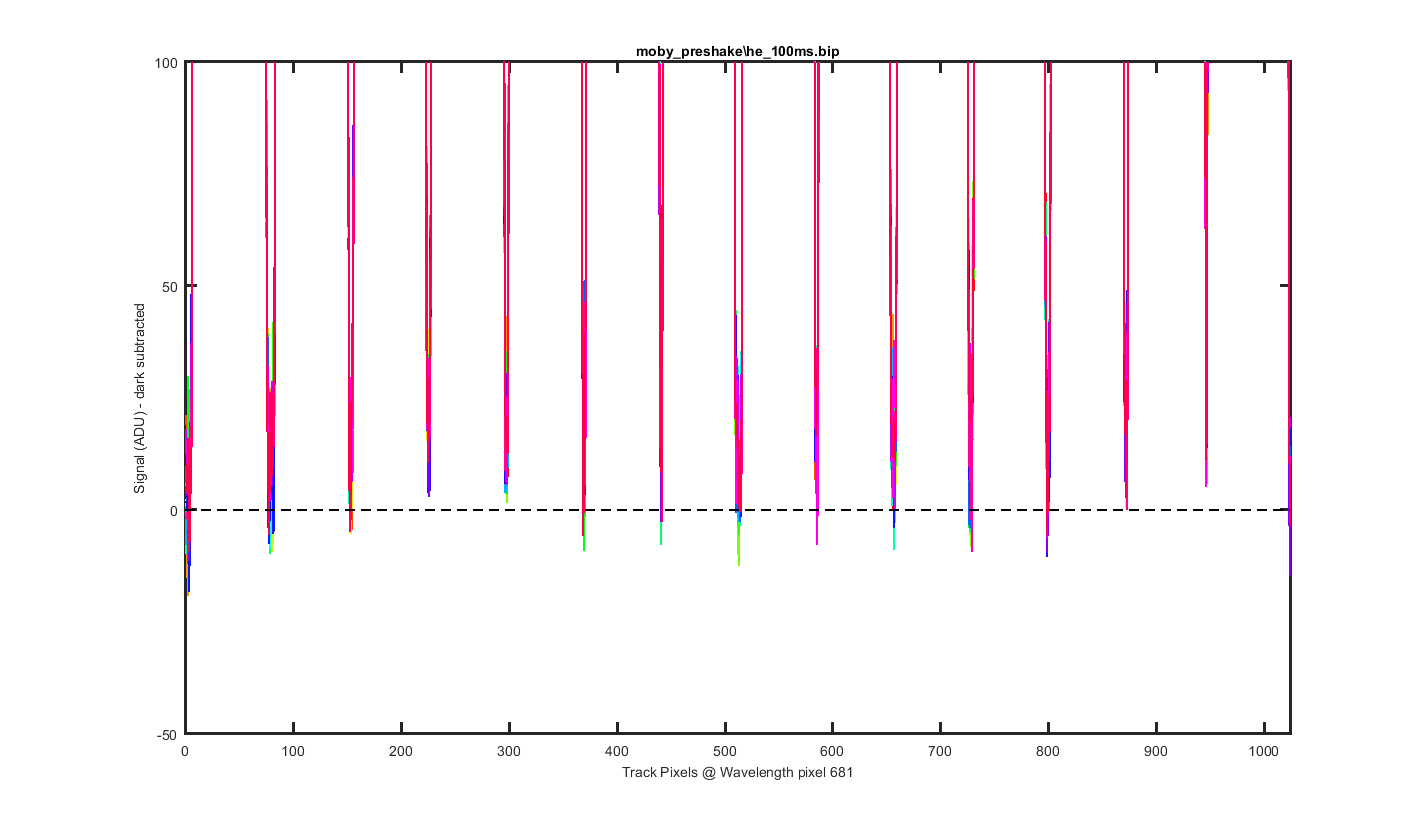
Figure 3
Same as the previous graph but zoomed into the bottom to see the level of the darks between the tracks.
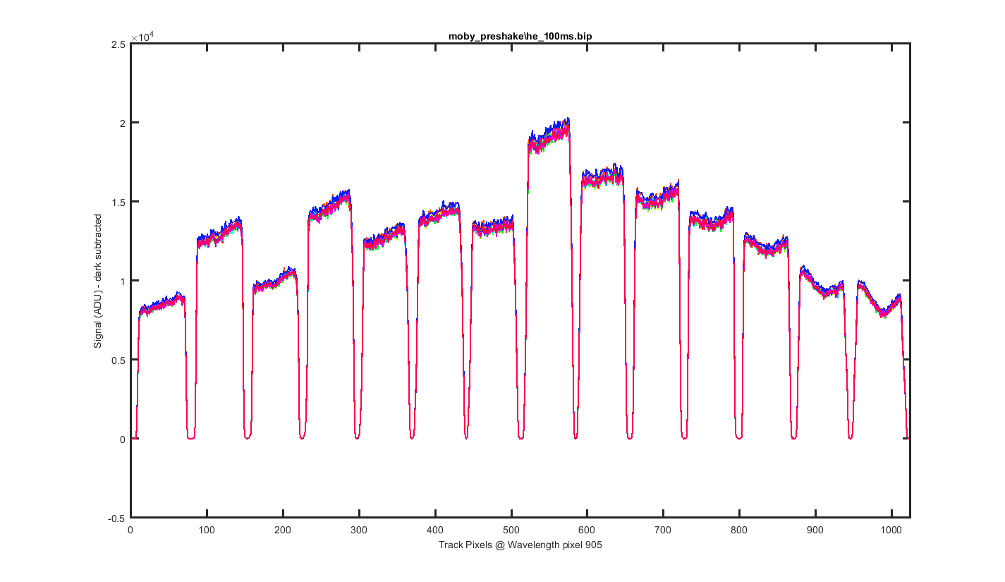
Figure 4
Same as figure 2 but for Wavelength pixel 930.
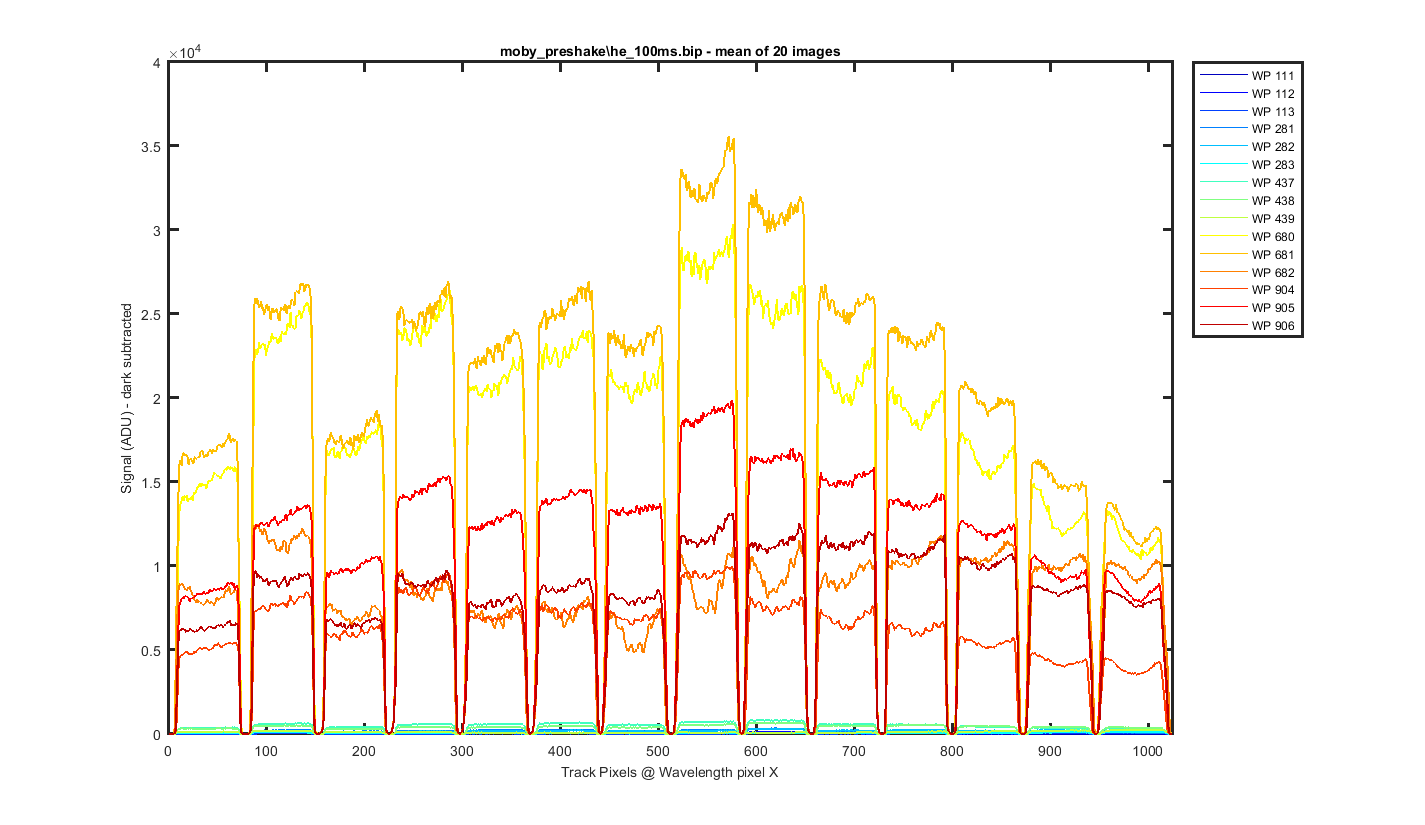
Figure 5
Again this is the mean image with slices thought the image at different wavelength pixels. The pixels choosen are where the helium peaks are and +- pixel pixel around them.
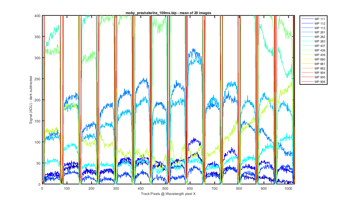
Figure 6
Same as figure 5 but zoomed to the bottom so you can see the darks between the tracks.
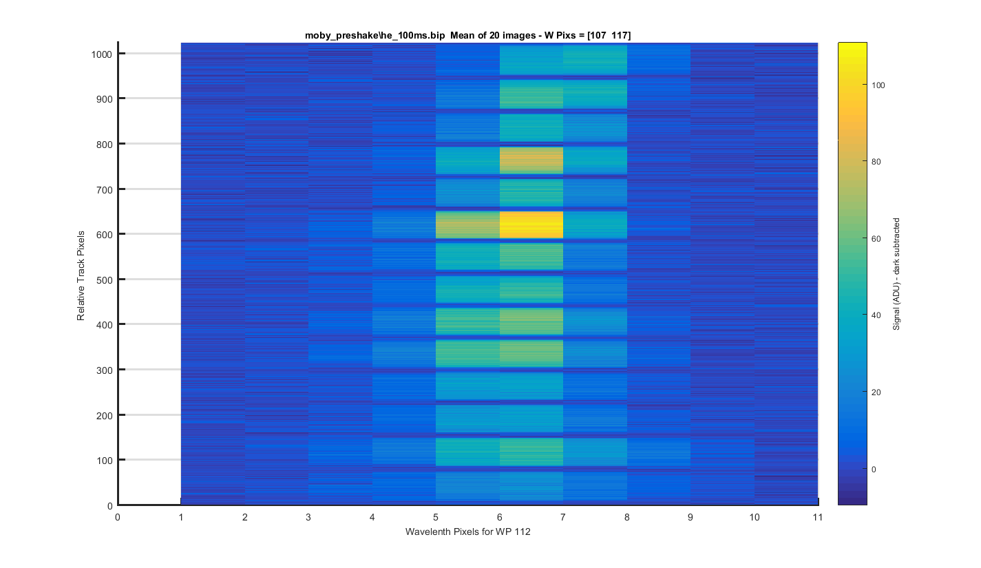
Figure 7
Helium Peak 1 (at pix 112): The same surface plot but showing how individual helium peaks line up from track to track.
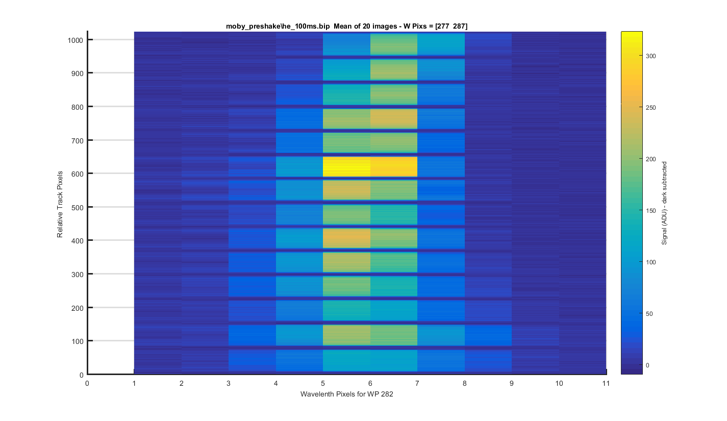
Figure 8
Helium Peak 2 (at pix 282): The same surface plot but showing how individual helium peaks line up from track to track.
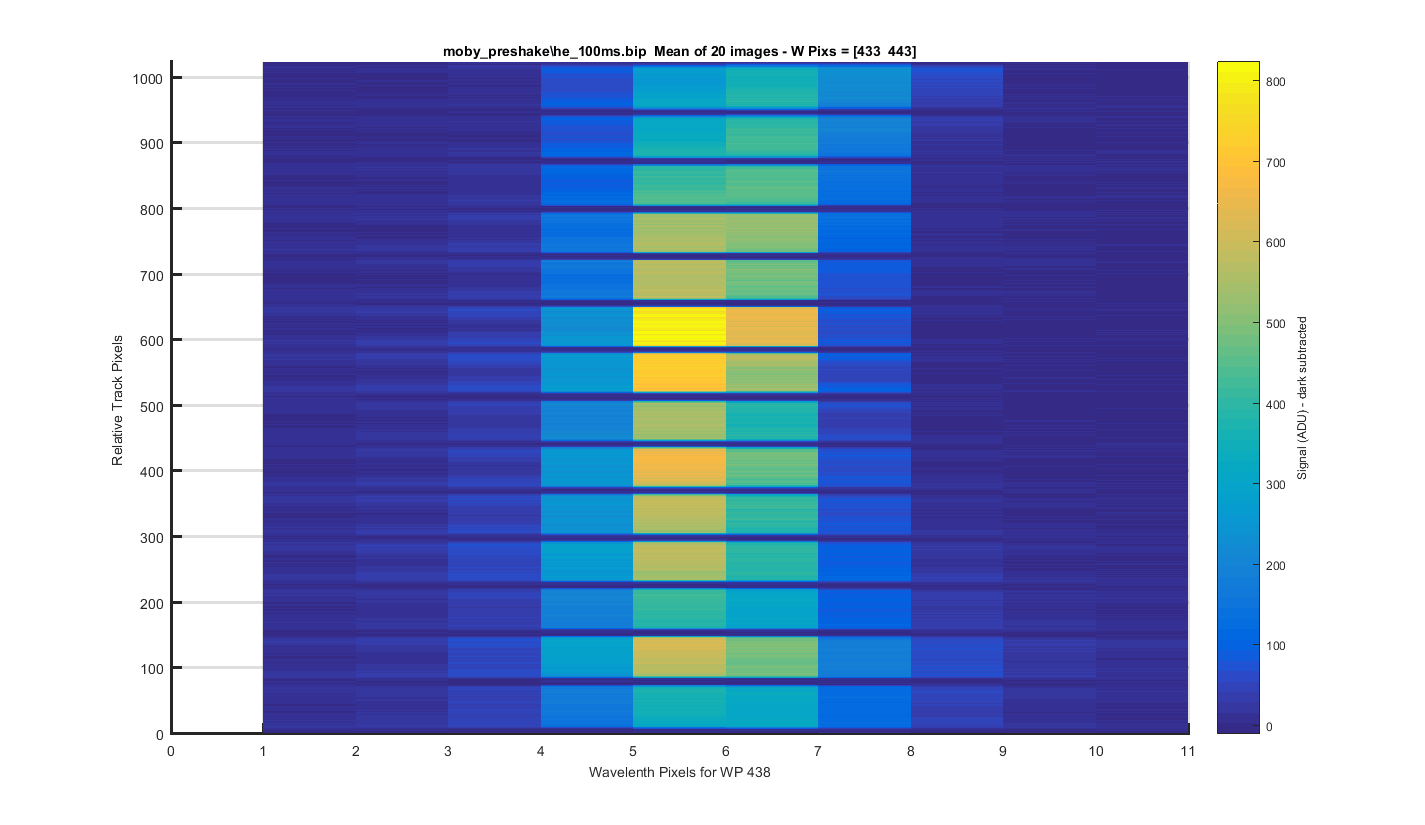
Figure 9
Helium Peak 3 (at pix 438): The same surface plot but showing how individual helium peaks line up from track to track.
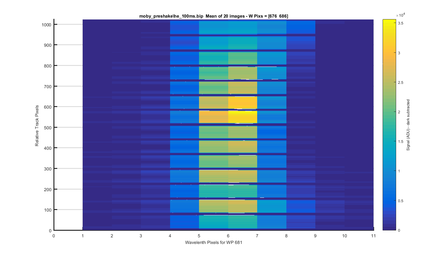
Figure 10
Helium Peak 4 (at pix 681): The same surface plot but showing how individual helium peaks line up from track to track.
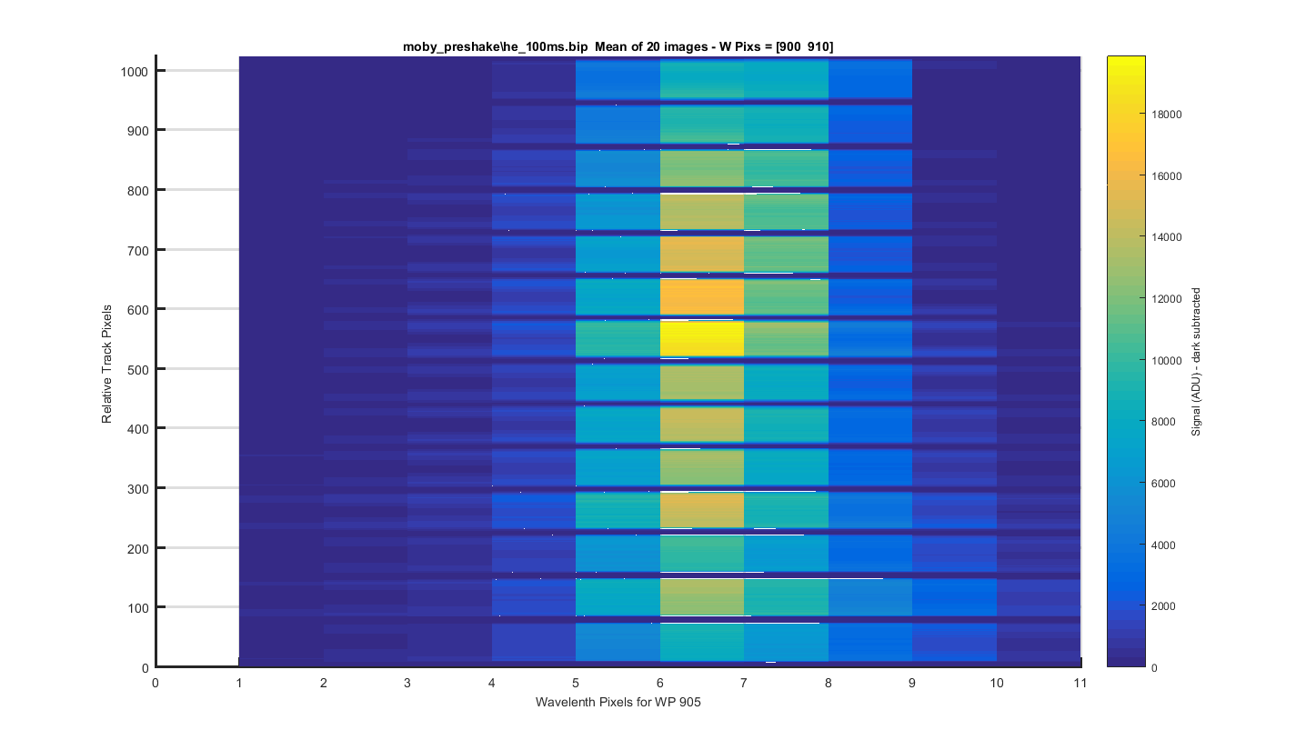
Figure 11
Helium Peak 5 (at pix 905): The same surface plot but showing how individual helium peaks line up from track to track.
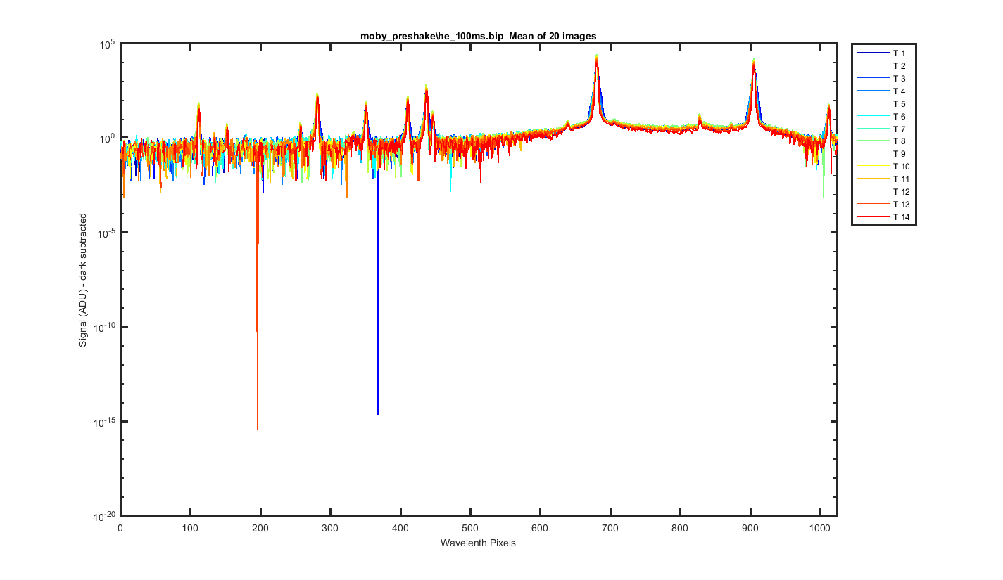
Figure 12
Mean image binned by track, the x-axis is wavelength pixels.
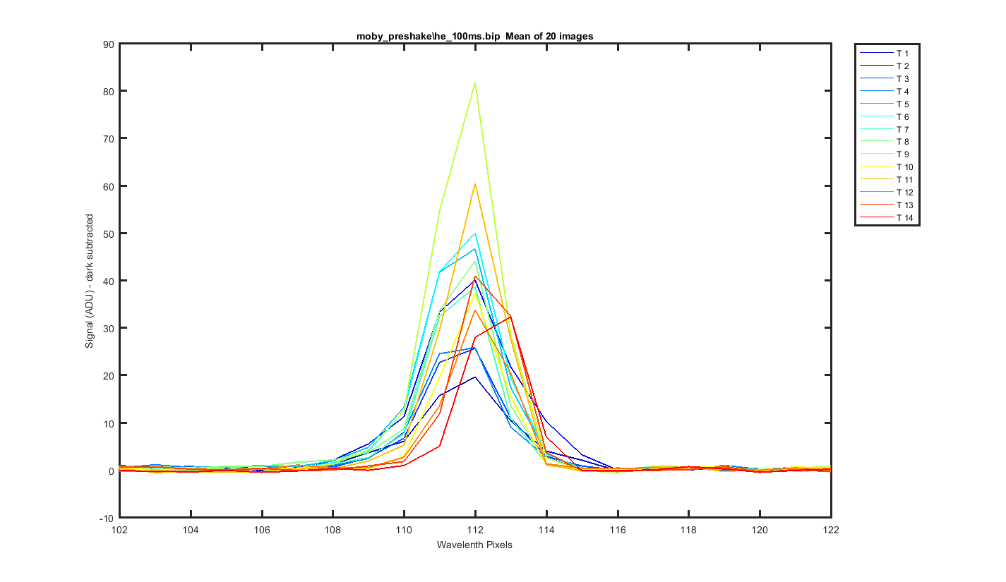
Figure 13
Close up of one of the helium peaks
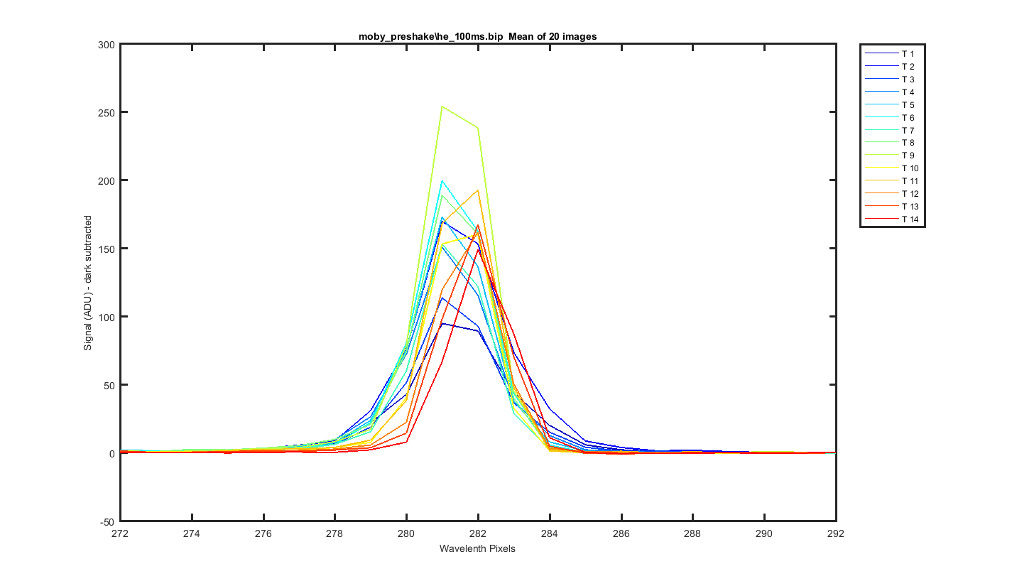
Figure 14
Close up of one of the helium peaks
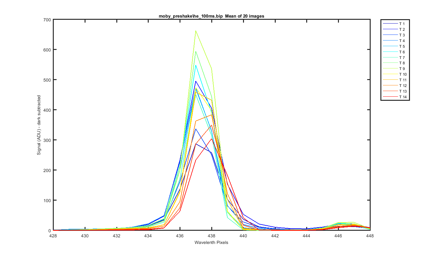
Figure 15
Close up of one of the helium peaks
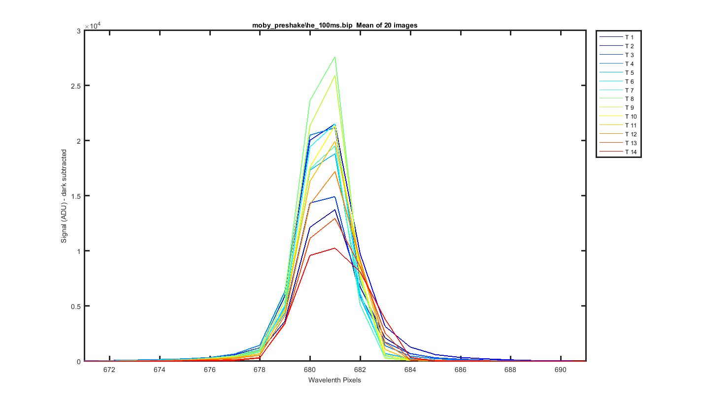
Figure 16
Close up of one of the helium peaks
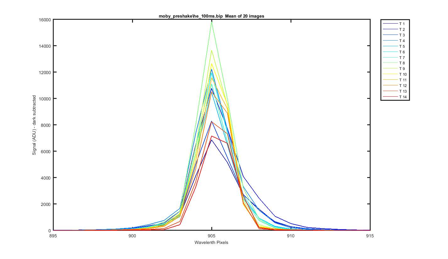
Figure 17
Close up of one of the helium peaks
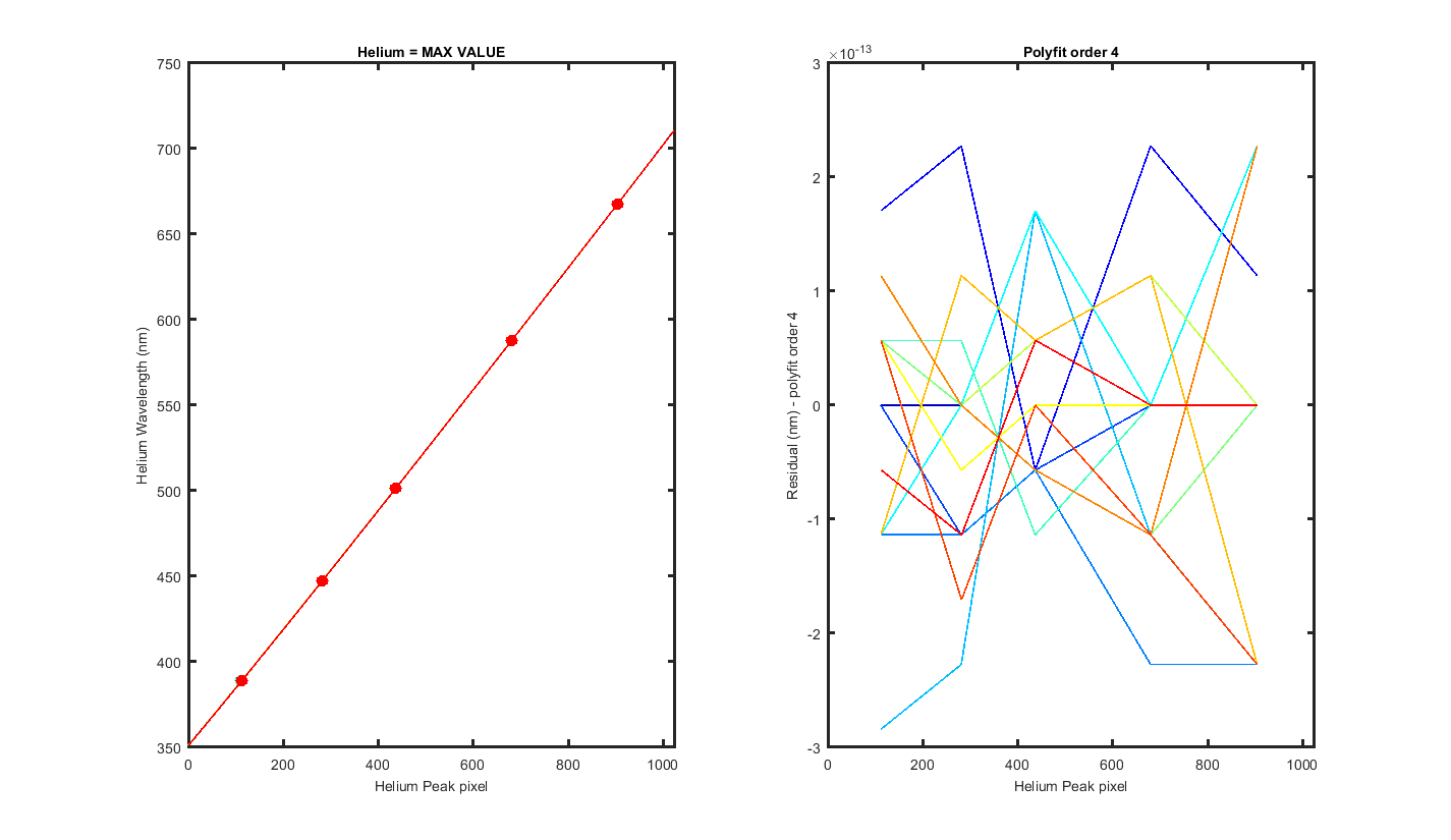
Figure 18
MY VERY ROUGH GUESS AT A WAVELENGTH CAL!!! THIS ASSUMES I GUESS CORRECTLY WHICH PEAKS WHERE WHICH HELIUM LINES.
Track, Min,    Max,     diff
    1, 351.55, 710.72,  0.35
    2, 351.50, 710.77,  0.35
    3, 351.66, 710.75,  0.35
    4, 351.69, 710.78,  0.35
    5, 351.63, 710.70,  0.35
    6, 351.60, 710.67,  0.35
    7, 351.60, 710.66,  0.35
    8, 351.52, 710.59,  0.35
    9, 351.55, 710.62,  0.35
   10, 351.40, 710.56,  0.35
   11, 351.48, 710.62,  0.35
   12, 351.38, 710.56,  0.35
   13, 351.30, 710.57,  0.35
   14, 351.25, 710.61,  0.35
  Track = The Resonon Track number
Lwave = Laser Wavelength
Lpix1 = Laser Pixel found using the max value of the track
Lpix2 = Laser Pixel found using mygaussfit to fit the laser peak
| Track | Lwave | Lpix1 | Lpix2 |
|---|---|---|---|
| 1 | 388.8648 | 112 | 111.81 |
| 1 | 447.148 | 281 | 281.48 |
| 1 | 501.5678 | 437 | 437.39 |
| 1 | 587.56 | 681 | 680.71 |
| 1 | 667.81 | 905 | 905.18 |
| 2 | 388.8648 | 112 | 111.91 |
| 2 | 447.148 | 281 | 281.47 |
| 2 | 501.5678 | 437 | 437.33 |
| 2 | 587.56 | 681 | 680.66 |
| 2 | 667.81 | 905 | 905.13 |
| 3 | 388.8648 | 112 | 111.65 |
| 3 | 447.148 | 281 | 281.36 |
| 3 | 501.5678 | 437 | 437.25 |
| 3 | 587.56 | 681 | 680.59 |
| 3 | 667.81 | 905 | 905.13 |
| 4 | 388.8648 | 112 | 111.54 |
| 4 | 447.148 | 281 | 281.26 |
| 4 | 501.5678 | 437 | 437.17 |
| 4 | 587.56 | 681 | 680.54 |
| 4 | 667.81 | 905 | 905.07 |
| 5 | 388.8648 | 112 | 111.59 |
| 5 | 447.148 | 281 | 281.28 |
| 5 | 501.5678 | 437 | 437.21 |
| 5 | 587.56 | 681 | 680.55 |
| 5 | 667.81 | 905 | 905.11 |
| 6 | 388.8648 | 112 | 111.64 |
| 6 | 447.148 | 281 | 281.32 |
| 6 | 501.5678 | 437 | 437.24 |
| 6 | 587.56 | 681 | 680.55 |
| 6 | 667.81 | 905 | 905.13 |
| 7 | 388.8648 | 112 | 111.62 |
| 7 | 447.148 | 281 | 281.30 |
| 7 | 501.5678 | 437 | 437.23 |
| 7 | 587.56 | 681 | 680.54 |
| 7 | 667.81 | 905 | 905.12 |
| 8 | 388.8648 | 112 | 111.69 |
| 8 | 447.148 | 281 | 281.33 |
| 8 | 501.5678 | 437 | 437.28 |
| 8 | 587.56 | 681 | 680.56 |
| 8 | 667.81 | 905 | 905.15 |
| 9 | 388.8648 | 112 | 111.78 |
| 9 | 447.148 | 281 | 281.45 |
| 9 | 501.5678 | 437 | 437.35 |
| 9 | 587.56 | 681 | 680.61 |
| 9 | 667.81 | 905 | 905.18 |
| 10 | 388.8648 | 112 | 111.93 |
| 10 | 447.148 | 282 | 281.46 |
| 10 | 501.5678 | 437 | 437.38 |
| 10 | 587.56 | 681 | 680.65 |
| 10 | 667.81 | 905 | 905.24 |
| 11 | 388.8648 | 112 | 111.98 |
| 11 | 447.148 | 282 | 281.59 |
| 11 | 501.5678 | 437 | 437.45 |
| 11 | 587.56 | 681 | 680.71 |
| 11 | 667.81 | 905 | 905.28 |
| 12 | 388.8648 | 112 | 112.15 |
| 12 | 447.148 | 282 | 281.71 |
| 12 | 501.5678 | 438 | 437.56 |
| 12 | 587.56 | 681 | 680.78 |
| 12 | 667.81 | 905 | 905.33 |
| 13 | 388.8648 | 112 | 112.34 |
| 13 | 447.148 | 282 | 281.88 |
| 13 | 501.5678 | 438 | 437.72 |
| 13 | 587.56 | 681 | 680.87 |
| 13 | 667.81 | 905 | 905.33 |
| 14 | 388.8648 | 113 | 112.59 |
| 14 | 447.148 | 282 | 282.10 |
| 14 | 501.5678 | 438 | 437.88 |
| 14 | 587.56 | 681 | 681.01 |
| 14 | 667.81 | 905 | 905.41 |