REVISION DATE: 25-May-2016 16:37:27

After plotting all the int time data on Page Num 100.02, I shall now try to simplify the graphs and look different regression schemes to fit the data. First simplification is I removed the duplicate 1 sec data. I left in the other duplicate int times (8 sec, 10 sec, etc). I have also reduced the number of tracks shows. I am only plotting Track 7 or track 1 or Track 14 , since these are the only tracks with collected with and with out cross track contamination. I also threw out day 5 is was a pain and seems to make the graphs harder to read. In the case where only one track is plotted the legend shows the day the data where collected. The Yes means the data are cross track contaminated and the No means they where not.

There are a couple of questions to be answered.

1. What type of line should we fit the data to?
2. What is the effect of cross track contamination, do we need to take the data on single tracks to get an acuarate calibration?
3. How different are the individual tracks (I.E. do we need a int cal for each track).

Track 7 data - light blue diamonds are the cross track contaminated (Yes) and the dark blue squares are the uncontaminated (No) data. There is also Day 4 data which are uncontaminted but hard to see. Using table curve 2D Mike found the "Power(a,b,b)" which is Y = a + b*X^c was the number one ranked fit. The fit is plotted as red lines for the Yes and No data. I should note that this fit is not forced through 1,1. But the best fit when you include polynomial fits is a 5th order fit (blue lines). The poly fit is forced through 1,1 which I think is correct. The ratio should be exactly one one nice that is what we are normalizing too. Just looking at the fit the 5th order poly does a better job everywhere but the goodness of the fit is most noticable at the higher int times. The r^2 are higher for the poly fit and the standard error is lower. So the rest of the graphs will show only the poly fit.

Figure 1

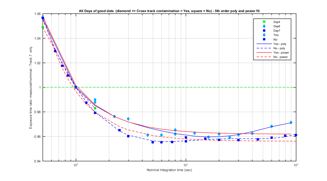
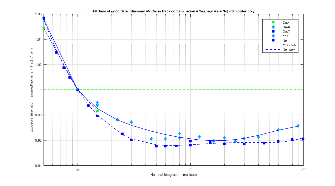
For track 7 there is about a 1% difference between the cross track contaminated and uncontaminated data.

Figure 2

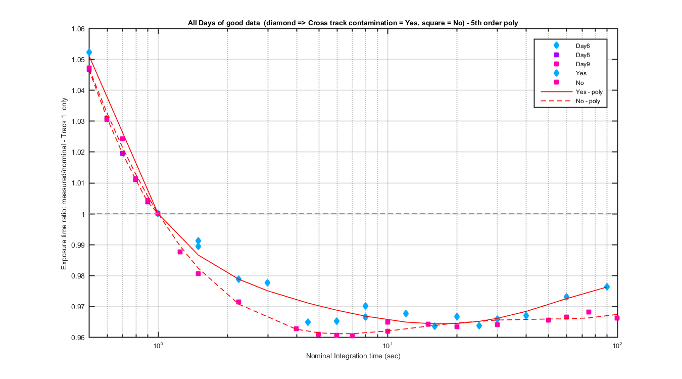
For track 1 there is also about a 1% difference between the cross track contaminated and uncontaminated data.

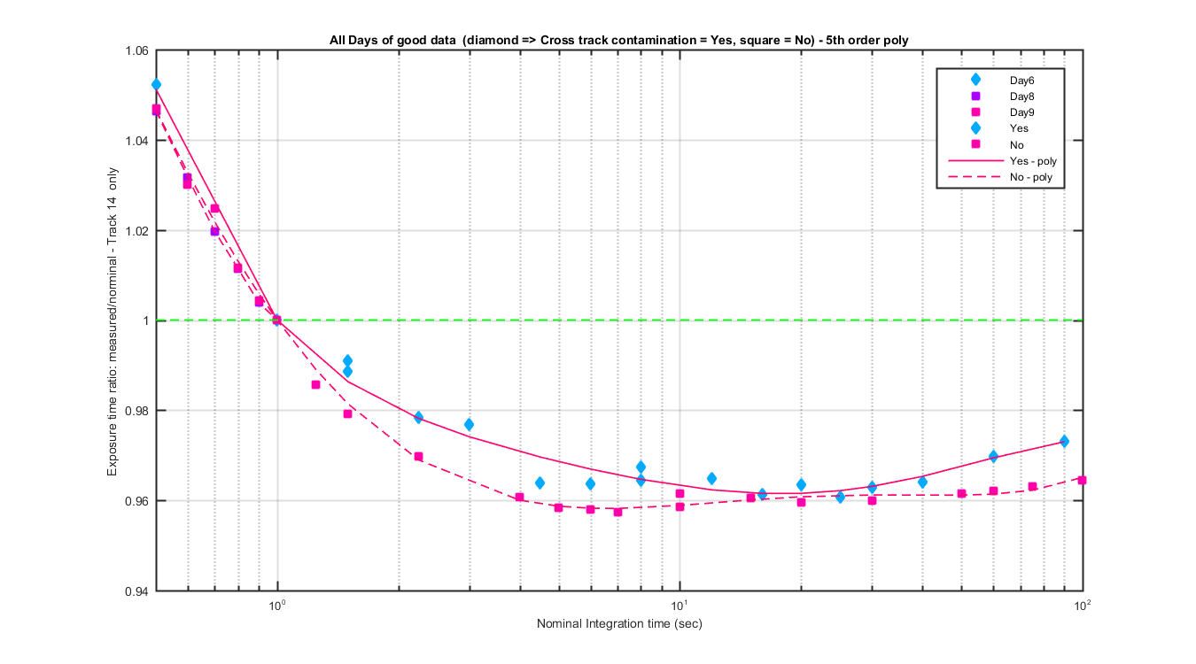
Figure 3

For track 14 there is also about a 1% difference between the cross track contaminated and uncontaminated data.

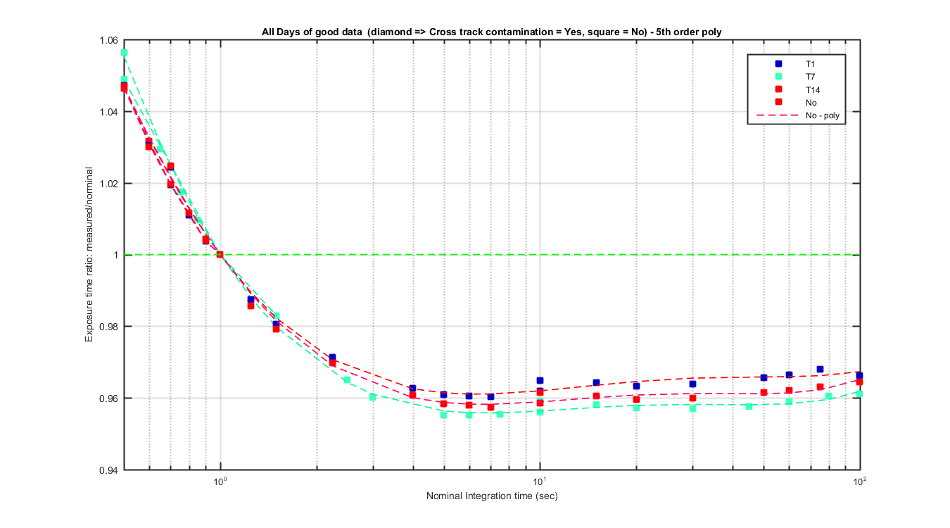
Figure 4

This is comparing the three uncontaminated tracks and their polt fit.

Figure 5

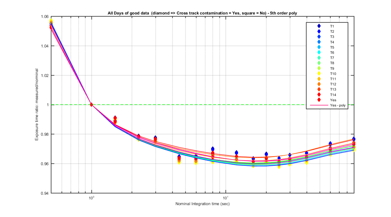
This is compares 14 contaminated tracks and their polt fit.

Figure 6