REVISION DATE: 13-May-2016 11:29:18

The data for this page are in ADU/pix/sec and they are all NET signals (lite-dark) .

Day 6 data are a repeat of the day 5 data ,except Mike is using a Iris to reduce the lamp level. Which is better than using the lamp voltage. Decreasing the lamp voltage changes the spectral shape of the light. Which we do not want. There are three lamp levels. High, Middle and Low (H,M and L in some legends). At the end of taking data for a specific lamp level there is a integration time repeat. Data is collected at say 1 sec a the high level, then the iris is closed a bit and the 1 sec data is repeated. Using these two repeats at the same int time but different light levels you can adjust the lower light level data to the higher. All the data were adjusted from the Low and Middle to the High. There is a second good way to do this using the PD monitor voltages. Which I show in a few graphs below, but the step down spectral ratios are better.

All the data where collected with all tracks on. This has large effect on the UV with the cross track stray light interpret that data with caution. Even though all the tracks are on makeing 14 track plots for each graphs would be nuts. So I mostly only plotted track 7 for the spectral graphs.

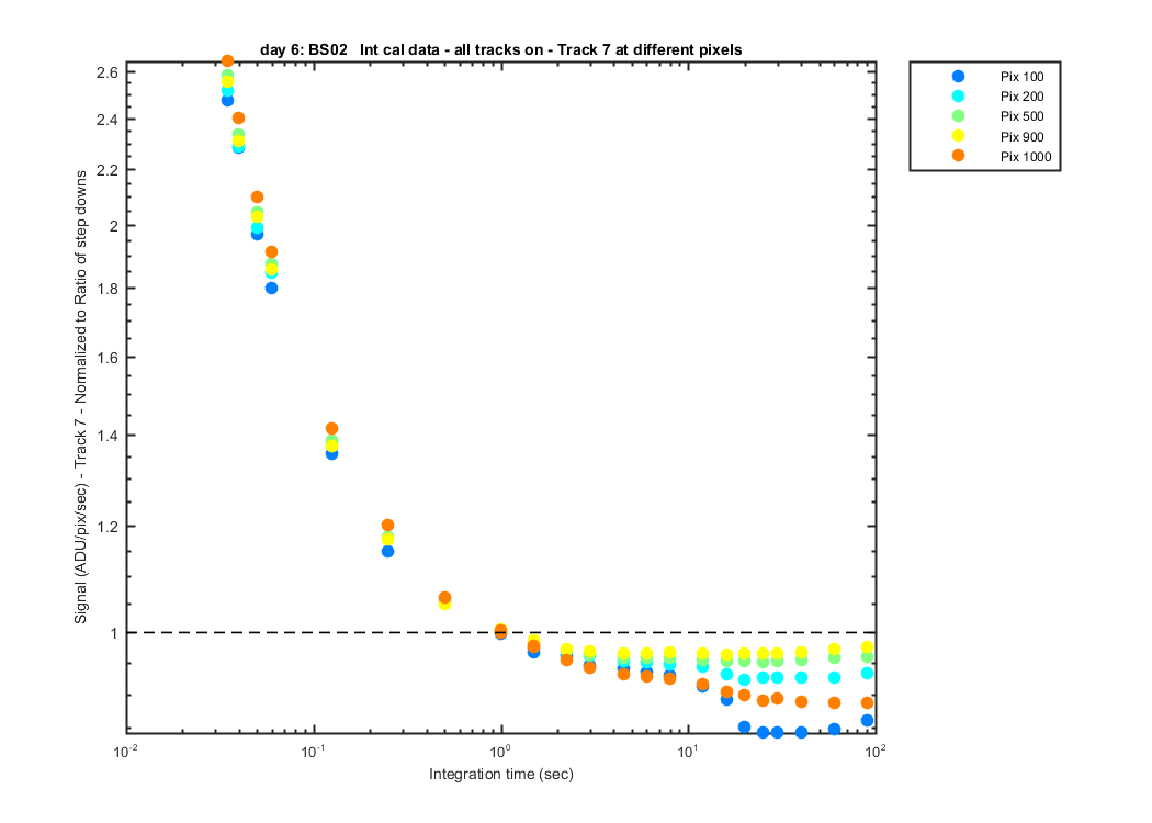
I then took the corrected data (using the step down spectral ratios) and calculated the 11 pix mean for pixels 100:100:1000. These data are plotted in various combinations of track and pixels.

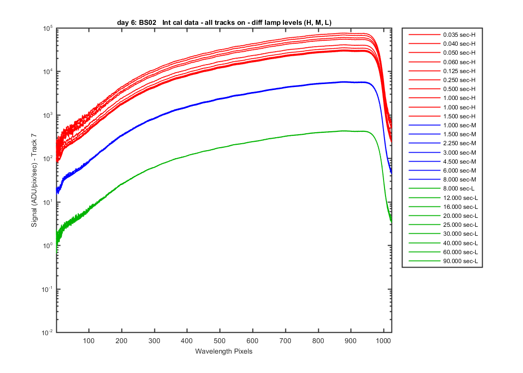
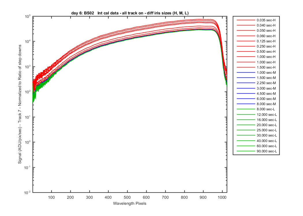
Track 7 data for all the data sets and lamp levels.

Figure 1

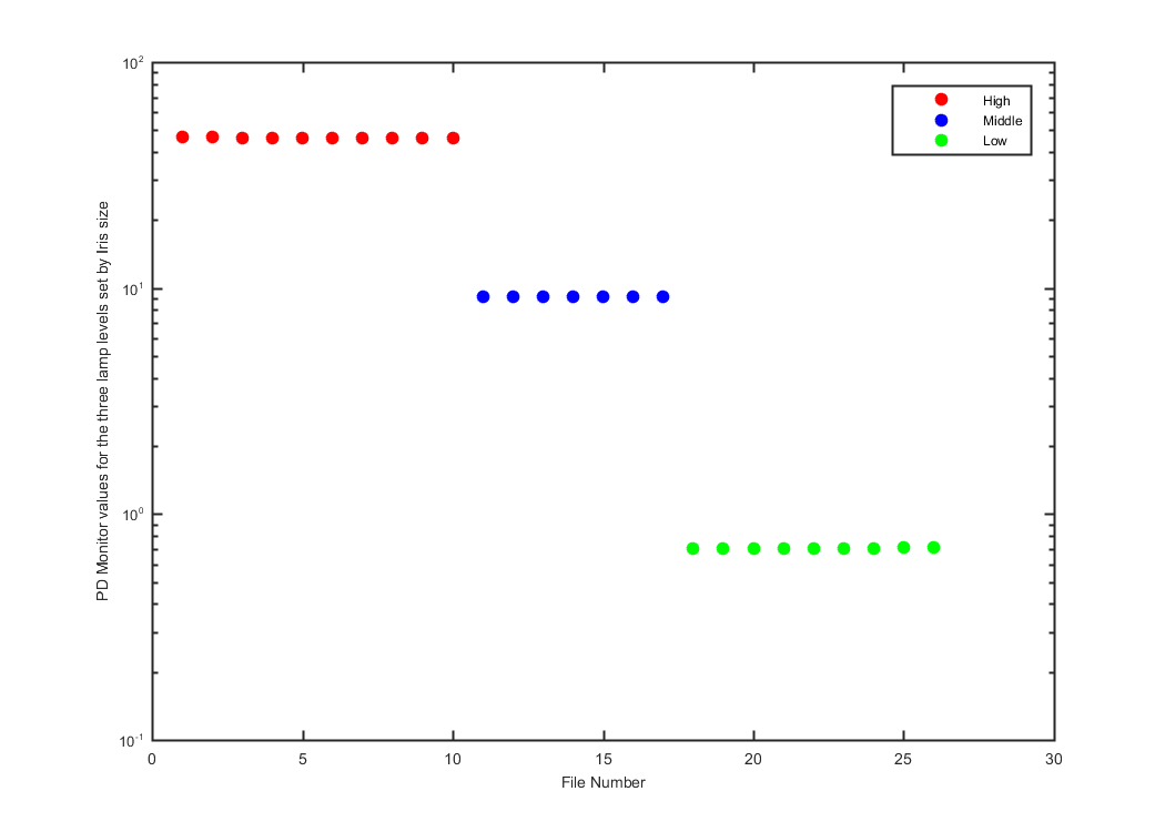
PD monitor values for the three lamp levels.

Figure 2

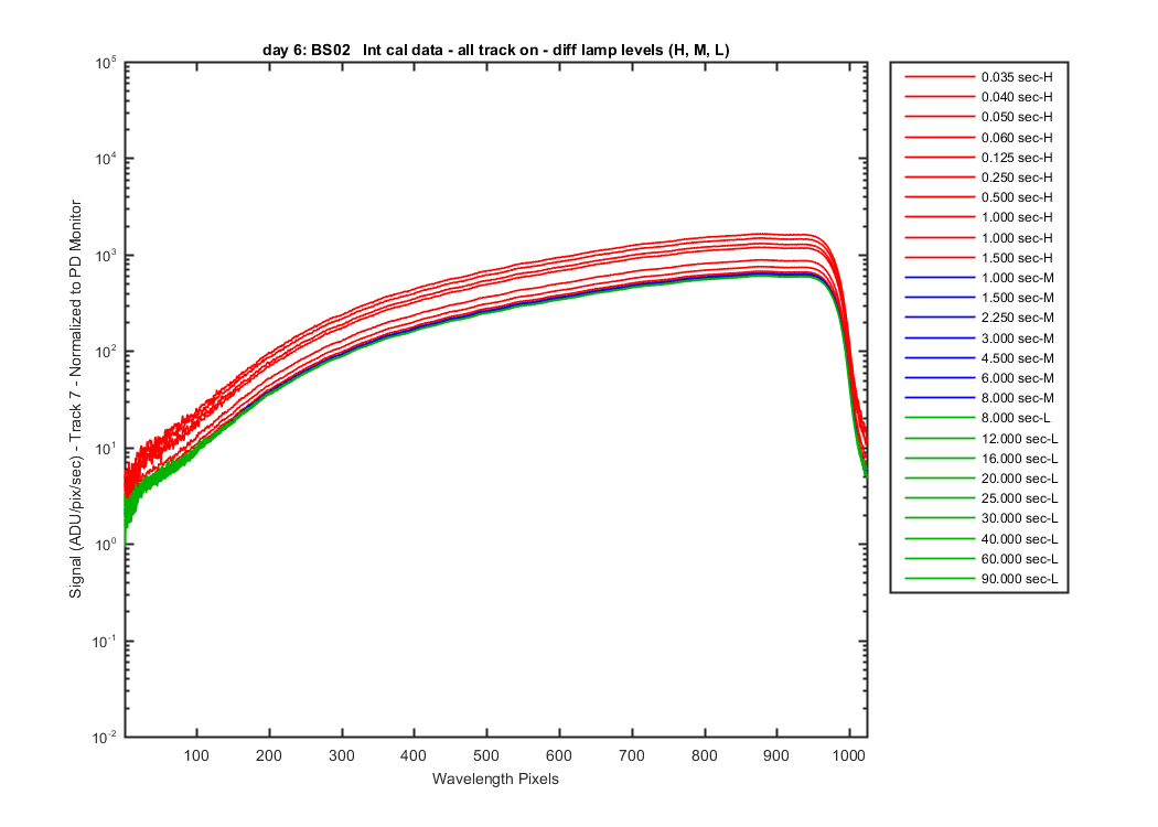
Lamp date normalized by the PD monitor values, just for fun.

Figure 3

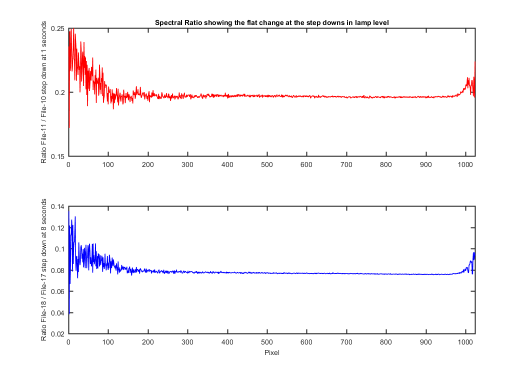
Ratios showing the change in the lamp level step downs from High to Middle (red line) and Middle to Low (blue line).

Figure 4

Track 7 data normalized using the step down ratios. I used a spectral ratio to do the correction, rather than one mean number.

Figure 5

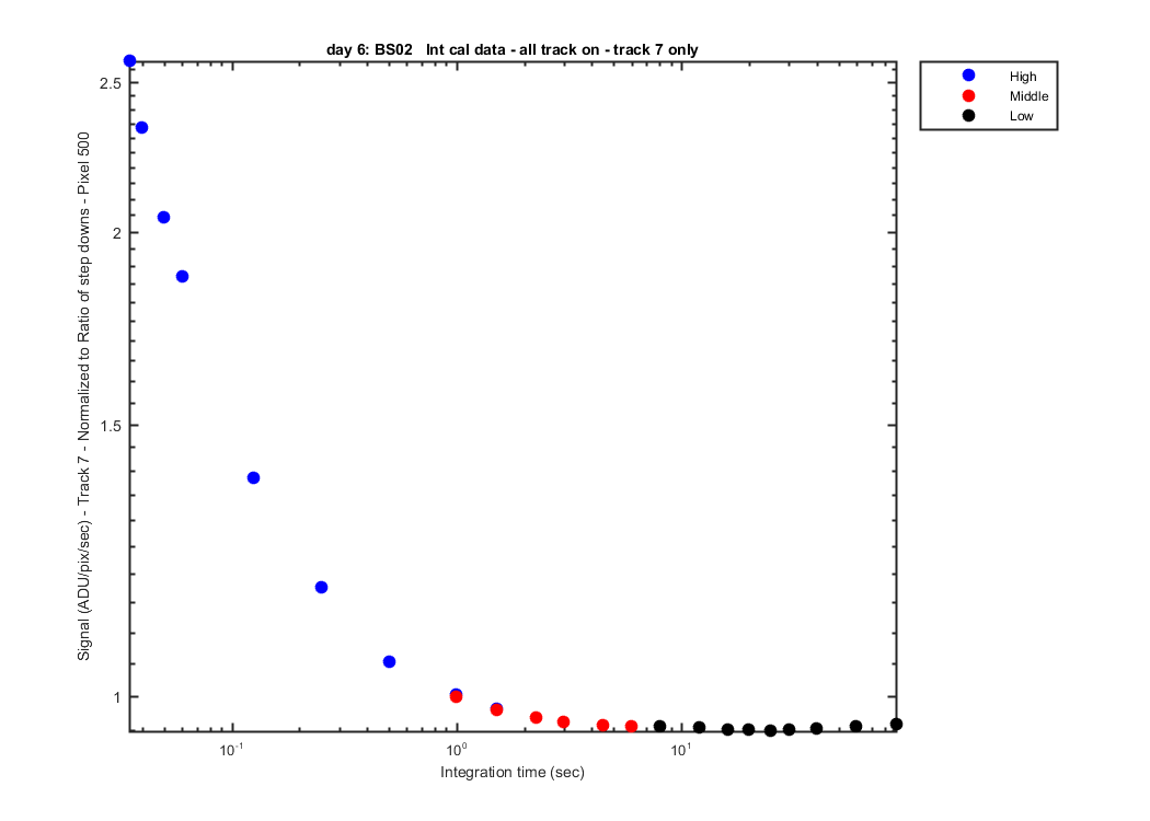
Track 7 data normalized (using the step down ratios) and then a 11 pixel mean at pixel 500 plotted version integration time. The colors show the different lamp levels

Figure 6

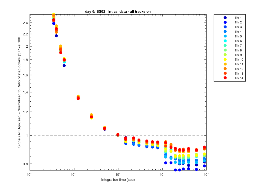
Same graph as above but for all the tracks at Pixel 100.

Figure 7

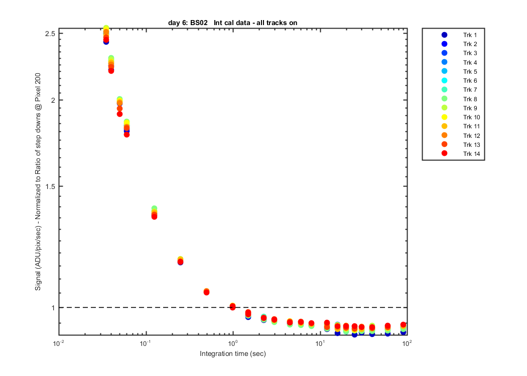
Same graph as above but for all the tracks at Pixel 200.

Figure 8

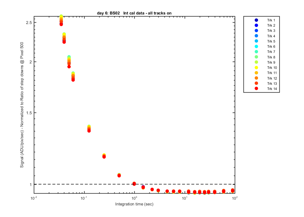
Same graph as above but for all the tracks at Pixel 500.

Figure 9

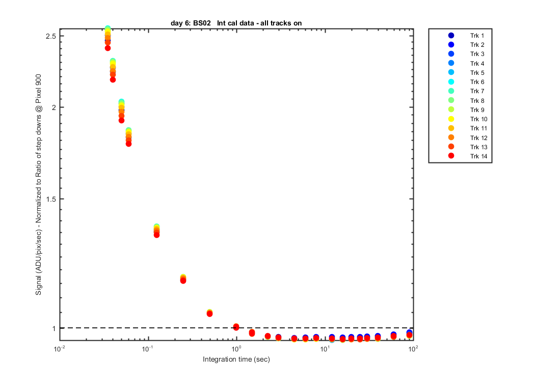
Same graph as above but for all the tracks at Pixel 900.

Figure 10

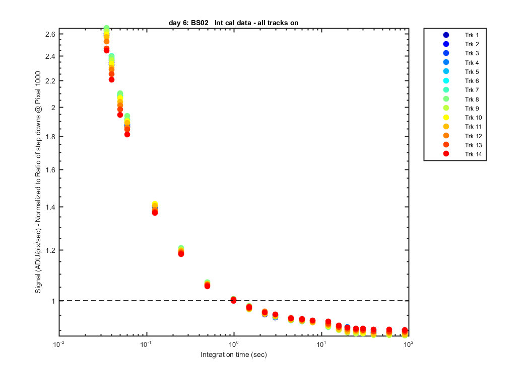
Same graph as above but for all the tracks at Pixel 1000.

Figure 11

Normalized Track 7 data again but with different pixesl compared

Figure 12