REVISION DATE: 23-Feb-2018 15:13:24
Mike did a quick exposure time cal. Using Mike detailed email and the int cal from MOBY-L264 day 7 I calculated a calibrated integration times. My method differed from Mikes in that I meaned all the 1 sec and 10 sec data so I normalized by the mean a 1 sec etc. See explainations below for more details about each step. Note: Data are in ADU/pix (the per pixel is because this is a track mean). They are all NET signals (lite - backgrounds)
Data listing M263pre_inttimecal.txt
fitresult =
     General model:
     fitresult(x) = a+b*x+c*x*log(x)+d./x^(0.5)
     Coefficients (with 95% confidence bounds):
       a =     0.06211  (0.04497, 0.07924)
       b =      0.9457  (0.9424, 0.949)
       c =    0.002427  (0.001713, 0.003141)
       d =   -0.004172  (-0.01185, 0.003504)
gof =
  struct with fields:

           sse: 0.0058
       rsquare: 1.0000
           dfe: 23
    adjrsquare: 1.0000
          rmse: 0.0159
| Precal Haw_2017-01 |
Postcal L264 |
||
|---|---|---|---|
| Nominal (sec) |
Measred (sec) |
Measred (sec) |
Post-Pre (sec) |
| 0.0500 | 0.0942 | 0.0973 | -0.0031 |
| 0.0700 | 0.1134 | 0.1149 | -0.0015 |
| 0.1000 | 0.1417 | 0.1428 | -0.0011 |
| 0.2000 | 0.2368 | 0.2387 | -0.0019 |
| 0.3000 | 0.3319 | 0.3328 | -0.0010 |
| 0.5000 | 0.5220 | 0.5224 | -0.0004 |
| 0.7000 | 0.7124 | 0.7126 | -0.0002 |
| 1.0000 | 1.0000 | 1.0000 | -0.0000 |
| 2.0000 | 1.9547 | 1.9493 | 0.0053 |
| 3.0000 | 2.9124 | 2.9002 | 0.0122 |
| 5.0000 | 4.8316 | 4.8060 | 0.0256 |
| 7.0000 | 6.7544 | 6.7163 | 0.0381 |
| 10.0000 | 9.6523 | 9.5847 | 0.0676 |
| 20.0000 | 19.2687 | 19.1196 | 0.1491 |
| 30.0000 | 28.8991 | 28.7002 | 0.1988 |
| 50.0000 | 48.2376 | 47.8003 | 0.4373 |
| 70.0000 | 67.6405 | 66.9453 | 0.6952 |
| 100.0000 | 96.8542 | 95.7781 | 1.0761 |
% File: \data\2017\L264\bs1cal\ascii_out\BS01_exptimecal(rev10Oct2017).txt
% Date: 10-Oct-2017;  by: MF/MLML
% What: 10-Oct-2017 post-MOBY262 BS01cfg007 LuBot Exposure Time Calibration via OL455-18U
%
% Contents:
% Column 1 = Nominal Exposure Time (sec)
% Column 2 = Calibrated Exposure Time (sec)
% Column 3 = Approximate Uncertainty in Calibrated Exposure Time (sec)
%
0.05    0.09759578  0.0009293666
0.07     0.1151779  0.0008480328
 0.1     0.1429966   0.000866055
 0.2     0.2390339   0.001162013
 0.3     0.3331735    0.00131359
 0.5     0.5228957   0.001516844
 0.7     0.7127801   0.001622318
   1             1             0
   2      1.946383    0.01011512
   3      2.898718    0.01545585
   5       4.80277    0.02441789
   7      6.712593    0.03479259
  10      9.586181    0.05889353
  20        19.097     0.1550128
  30      28.62378      0.278212
  50      47.91934      0.420614
  70      67.10489     0.6688524
 100      96.00898      1.027457
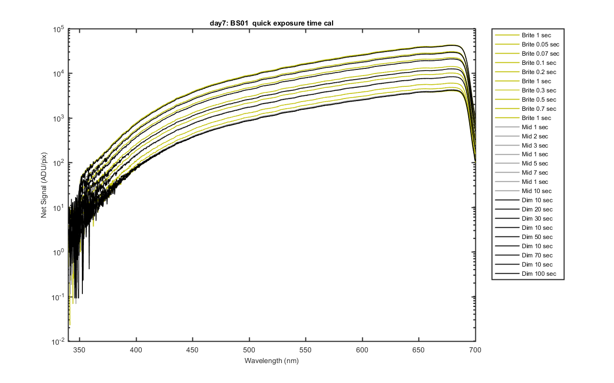
Figure 1
The data where collected a three different lamp levels ("Brite", "Mid", and "Dim") to be able to get a full range of integration times. You can see all the levels here.
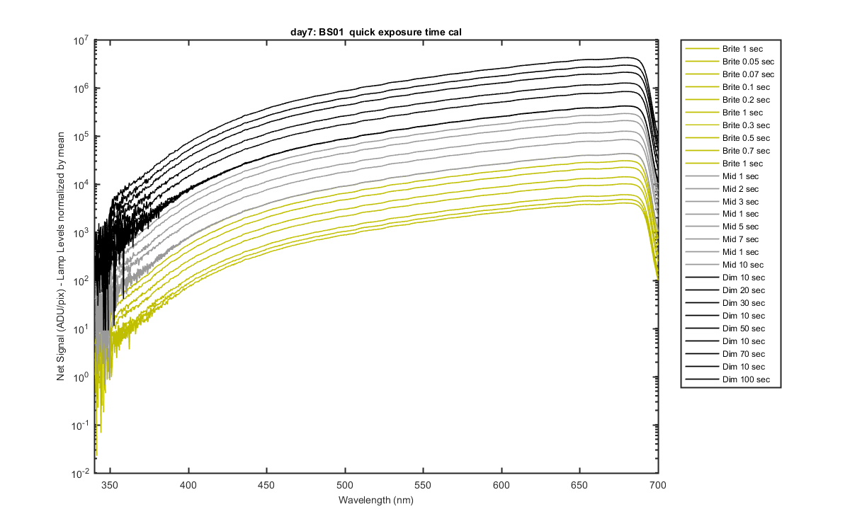
Figure 2
Track 13 data normalized using the step down ratios. So the 1 sec repeats from Bright to Mid and the 10 sec repeats from Mid to Dim plot on top of each other.
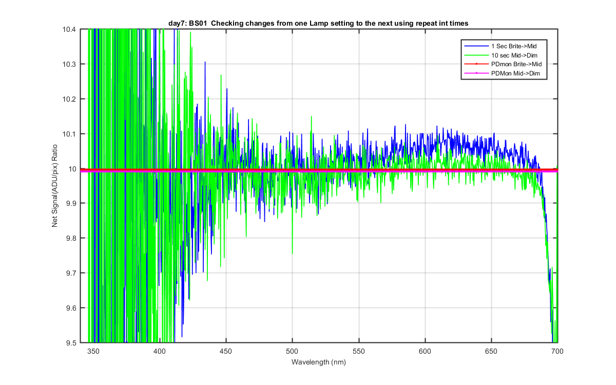
Figure 3
I am not totally sure what this graph is showing but I copied it from Mikes email. Email section below: I checked the Net Sig repeats at 1 sec for the Brite lamp (+/- 0.5%), and at 1 sec for the Mid lamp (+/- 1%), and at 10 sec for the Dim lamp (+/- 1.5%).Since they seemed OK, and the PD mon repeats were essentially 1, I did my Net Sig "normalizing" to the nearest-in-time 1 sec exposure Net Sig at Brite & Mid lamp settings, and to the nearest-in-time 10 sec net at Dim lamp setting(hopefully this will make sense below!). Yea, it looks the same as Mikes, now I need to understand what we are checking for here.
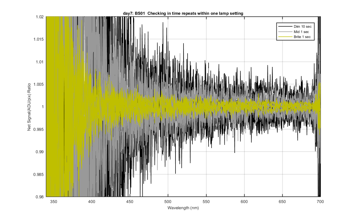
Figure 4
Checking the integration time repeatability within each lamp level. So I found all the Brite 1 sec and divided by the mean to get the variation about the mean. I did the same for the 1 sec Mid and 10 sec Dim data. This looked really good.
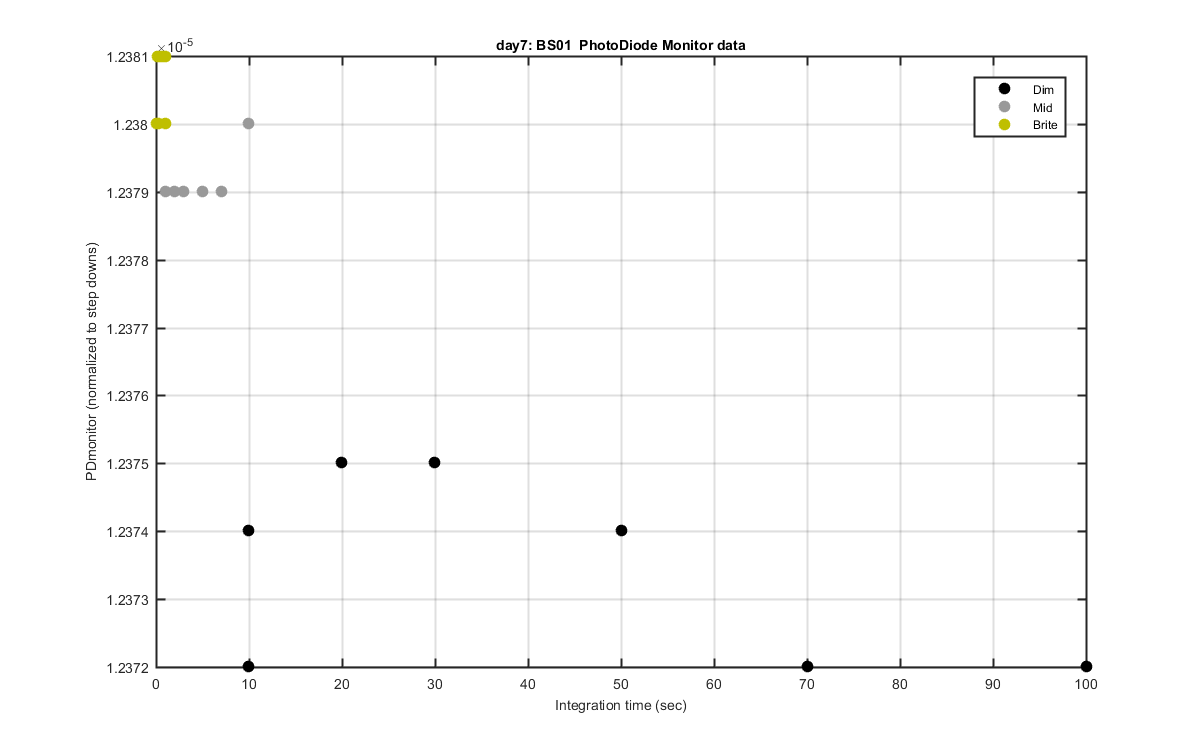
Figure 5
The Photodiode data normalized to the level changes using PDmonitor data.
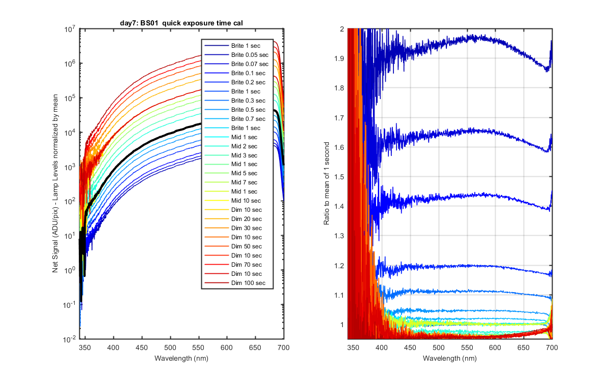
Figure 6
The left panel is the Same data from Figure 2. The right panel is each int time divided by the mean 1 sec data and integration time. I then calculated the mean for each ratio from pixels 300-900 and a std.
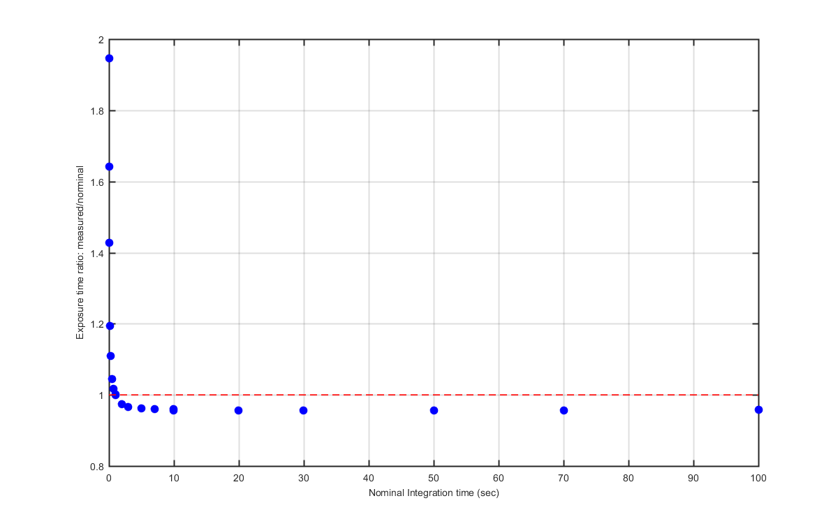
Figure 7
A plot of the ratio of measured over nominal Exposure time.
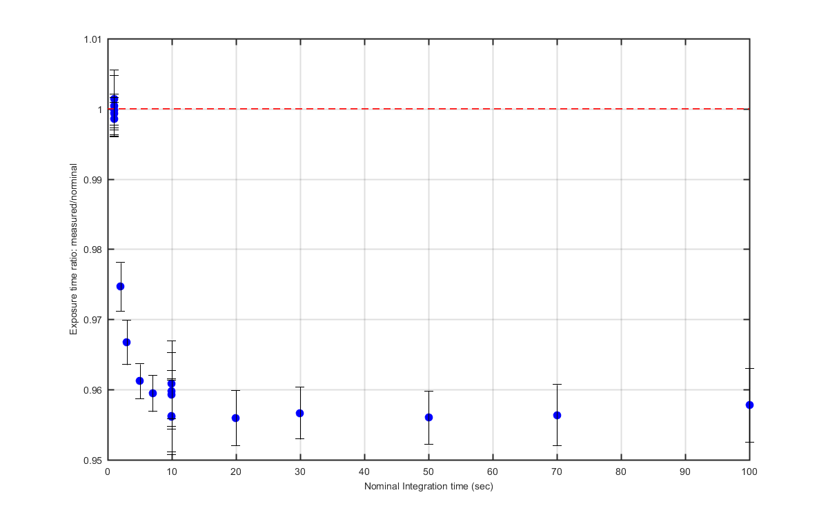
Figure 8
Zoomed in to the higher int time numbers with error bars.
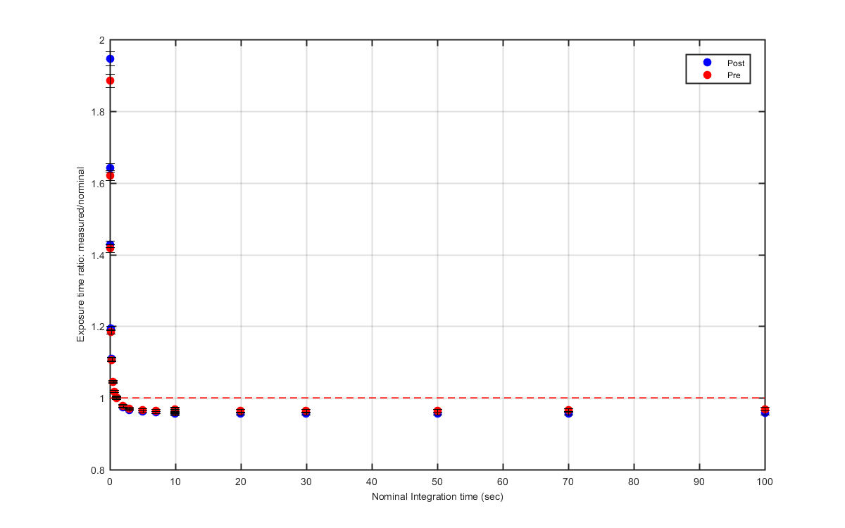
Figure 9
Comparison of predeployment int cal (my version) and the post deployment int cal (my version)
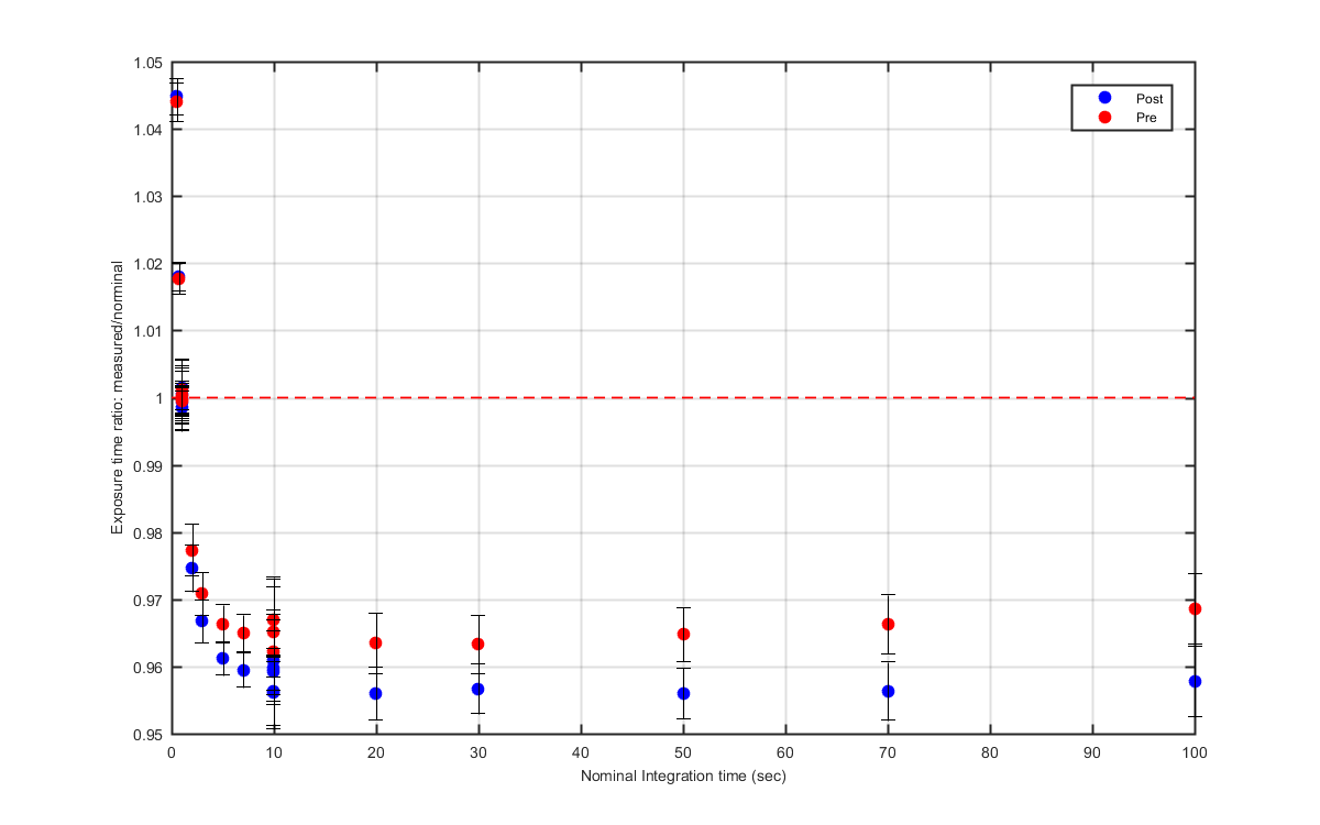
Figure 10
Same graphs as above but zoomed in
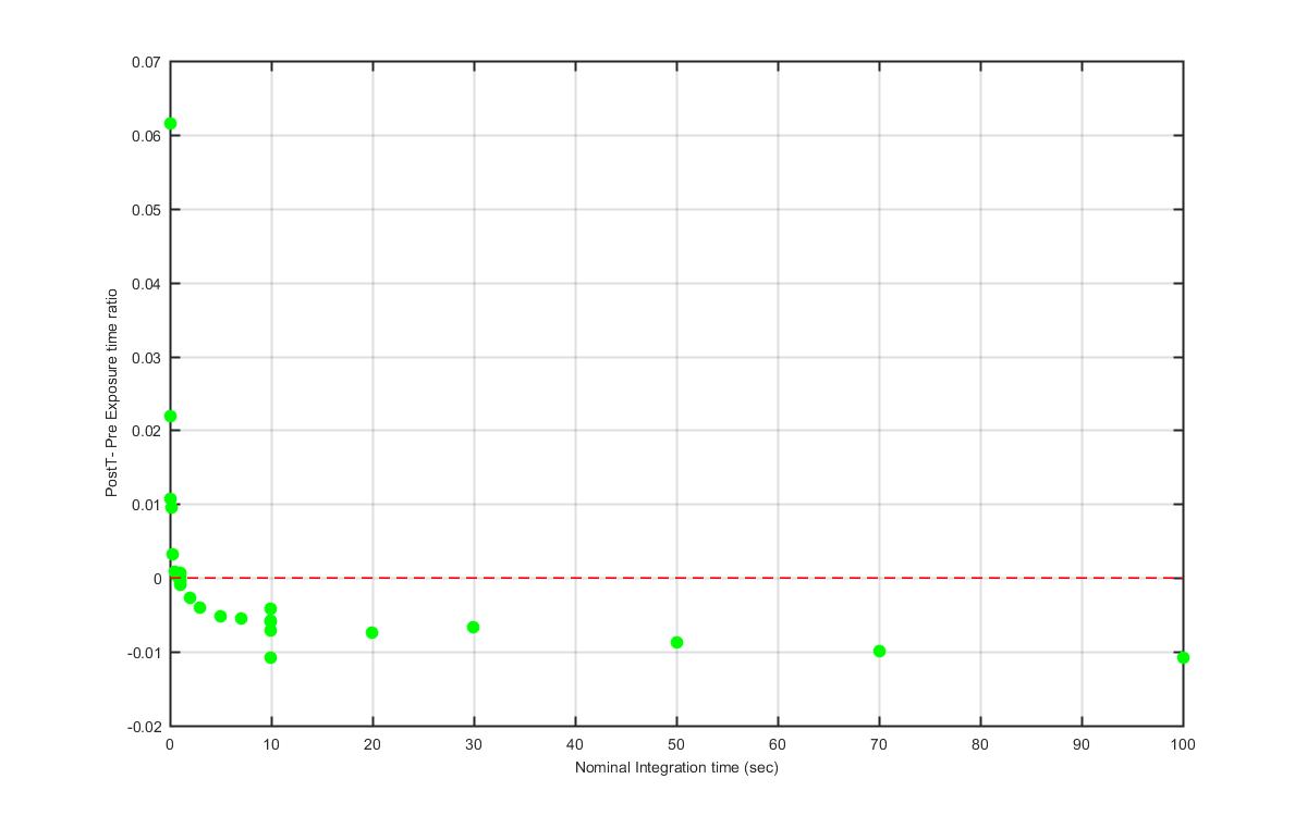
Figure 11
Difference between the post and pre deployment int cal
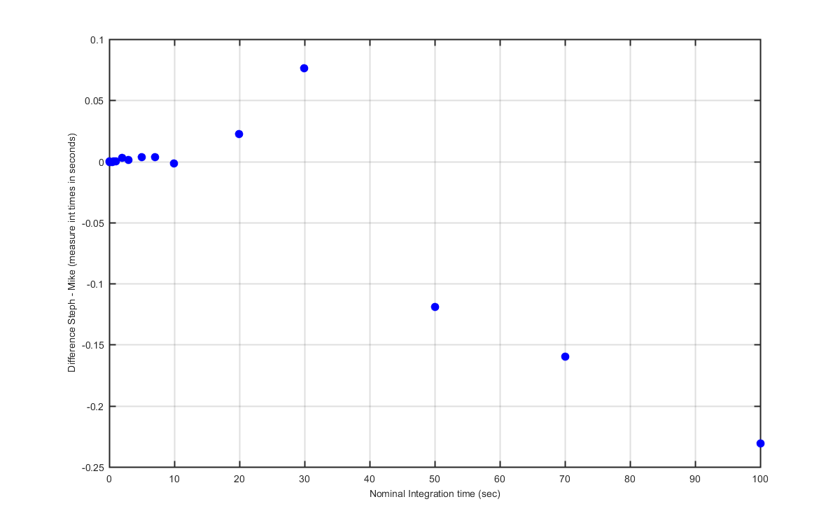
Figure 12