REVISION DATE: 02-Apr-2019 19:40:56
Wavelenght calibration using 5 Pen Lamps. All net files in the processing dir are loaded up and data not marked as wavelength calibration are removed. This program assumes and intial wavelength calibration that is good with int ~5 pixels. Next each lamp and line is evaluated to see if there is a peak very close by. The program them loops through each data set. This is using the "3 data set numbers" and track and and source info. Using the intial wavecal the peak is pulled out of the data set and the highest 2 peaks are returned. If there is a peak very close by then code determines if we want the first or second peak. For the Ne Lamp lines 13 and 18 code to modify the pixels used to pull out the peak. This fixed a problem with these peaks in 3 tracks. findpeaks is the funtion that returns the 2 highest peaks. It also returns peak value, location, width, and promenece. Once I have the right peak pulled out I use the location of the peak max and the peak width to pull out just the peak for the gaussian fit. I use fit with the gauss1 fittype input and the data. The fit coefficients and goodness of fit (GOF) values are returned. All these values, data, peak location, and peak are saved in a MLdbase file.
Once all the peaks have been found and the center pixel calculated from the gauusian fit it is time to do the wavecals for each track. I first remove outliers by doing a poly2 fit using the fit funtion and flagging any file with residuals greather than 1 nm. This is how I found the problem lines for Ne Lamp. The fit coeff are saved to the MLdbase file. Because there is some curve still in the fit data I then repeat the fit using poly 3 and save those coeff as well. The paragraph below shows the fitted data for each of the two types of fit.
2nd order Poly
P(13,:) = [1.103386e-05 0.3399184 337.4118];
3nd order Poly
P(13,:) = [-3.387284e-09 1.677827e-05 0.3371351 337.7383];
Pen Lamp used and wavelength of the lines
Lamp: HgA --> Wavelengths: [365.0158 404.7 407.8 435.8 491.6 546.1 577 579.1];
Lamp: Ne --> Wavelengths: [503.8 508 511.7 540.1 556.3 565.7 569 585.2 588.2 594.5 603 609.6 616.4 621.7 626.6 633.4 650.7 653.3 659.9 667.8 671.7 692.9];
The first graph below is the wavelenght cals for track 13. The Right graph shows the residuals. The second graph show all the lamp data and the dashed lines are the pen lamp lines for each lamp. The ones with symbols at the top and bottom of the graph are the pairs with very close peaks. The next group of graphs show each lamps net data with each lamps lines highlighted in grey with a red * at the top and a line numbers. A red patch means the data where flagged at having residual > 1 nm. The next group shows the indivdual gaussian fits for each lamp and lamp line. The title have the track number, line number and peak center pix from the gaussian fit. The last group shows the gaussian goodness of fit (GOF) data for each lamp and lamp line. Not sure what to do with these yet, but figured plotting them was better than not plotting them.
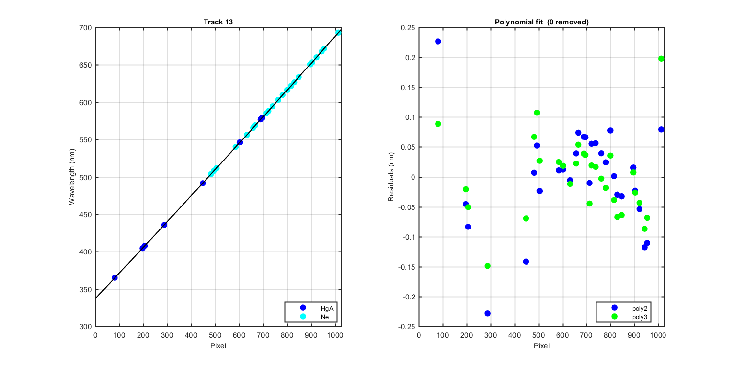
Figure 1
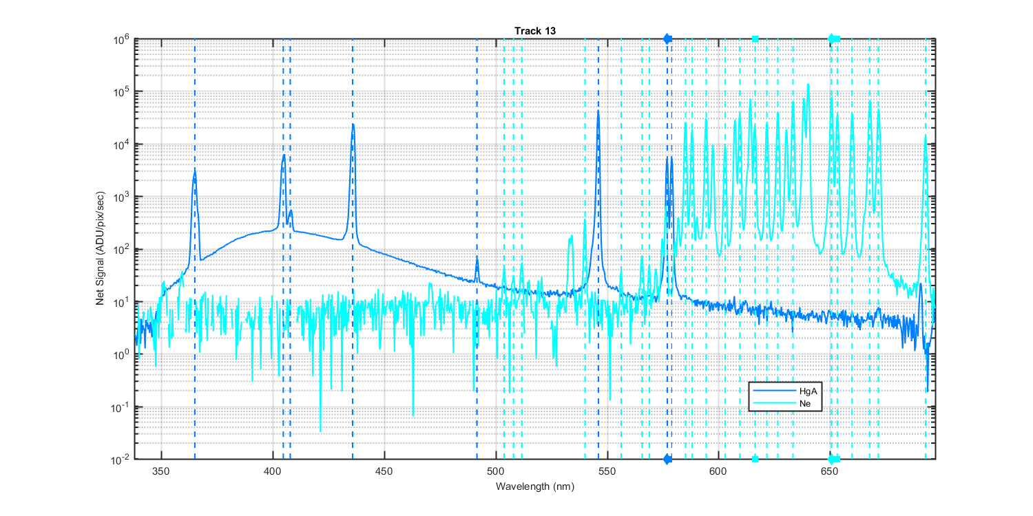
Figure 2
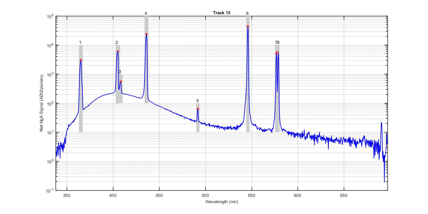
Figure 3
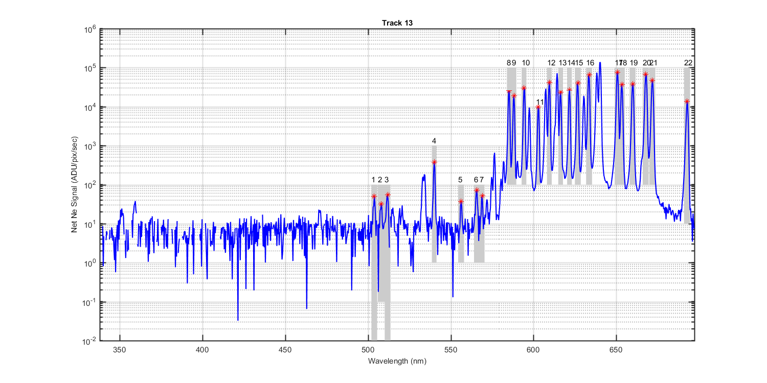
Figure 4
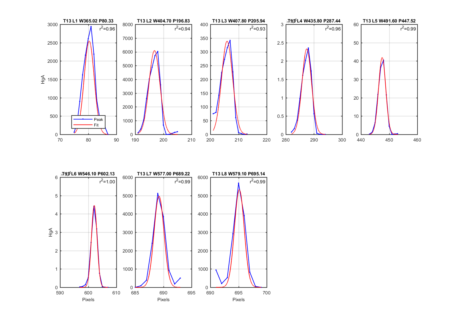
Figure 5
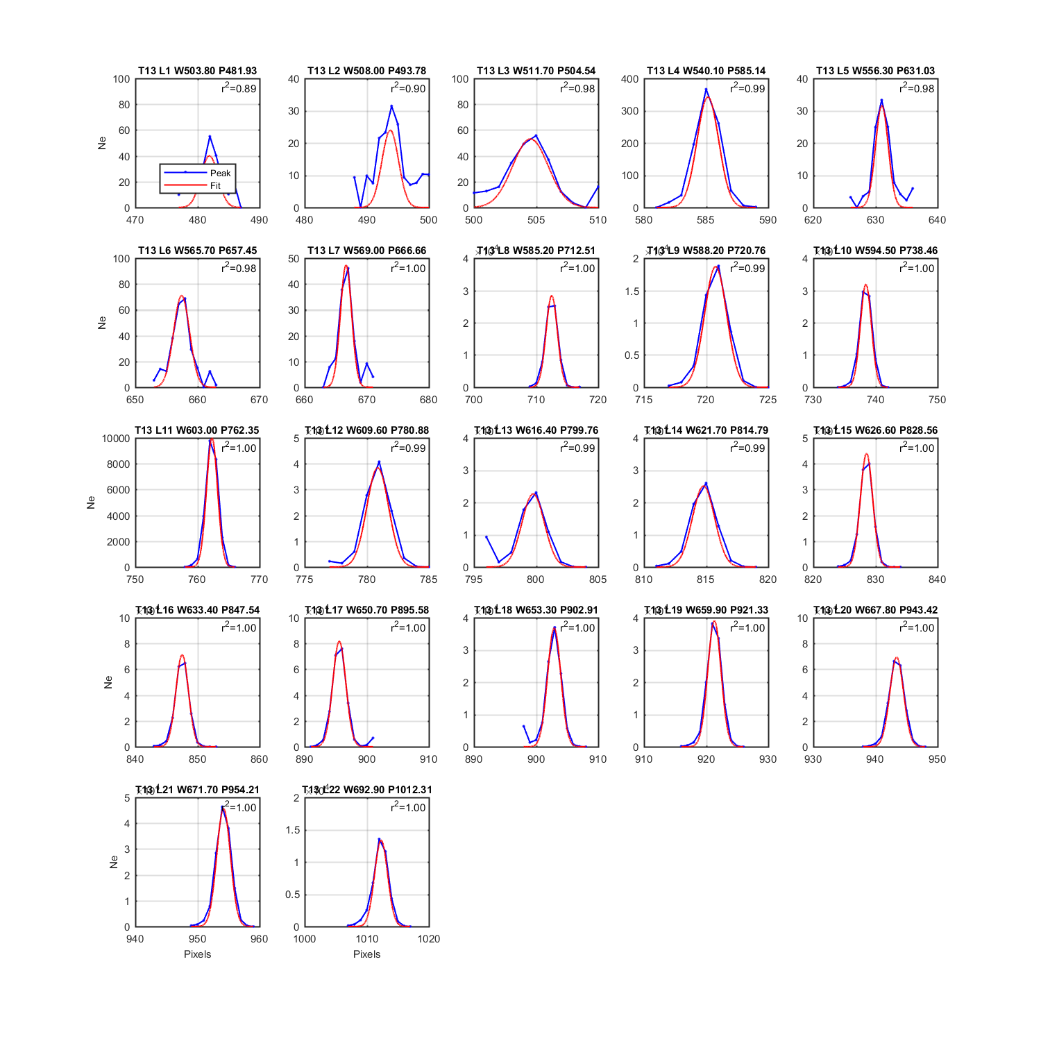
Figure 6

Figure 7
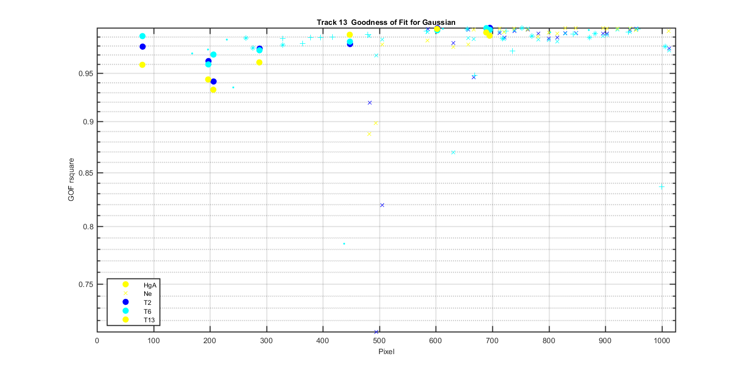
Figure 8
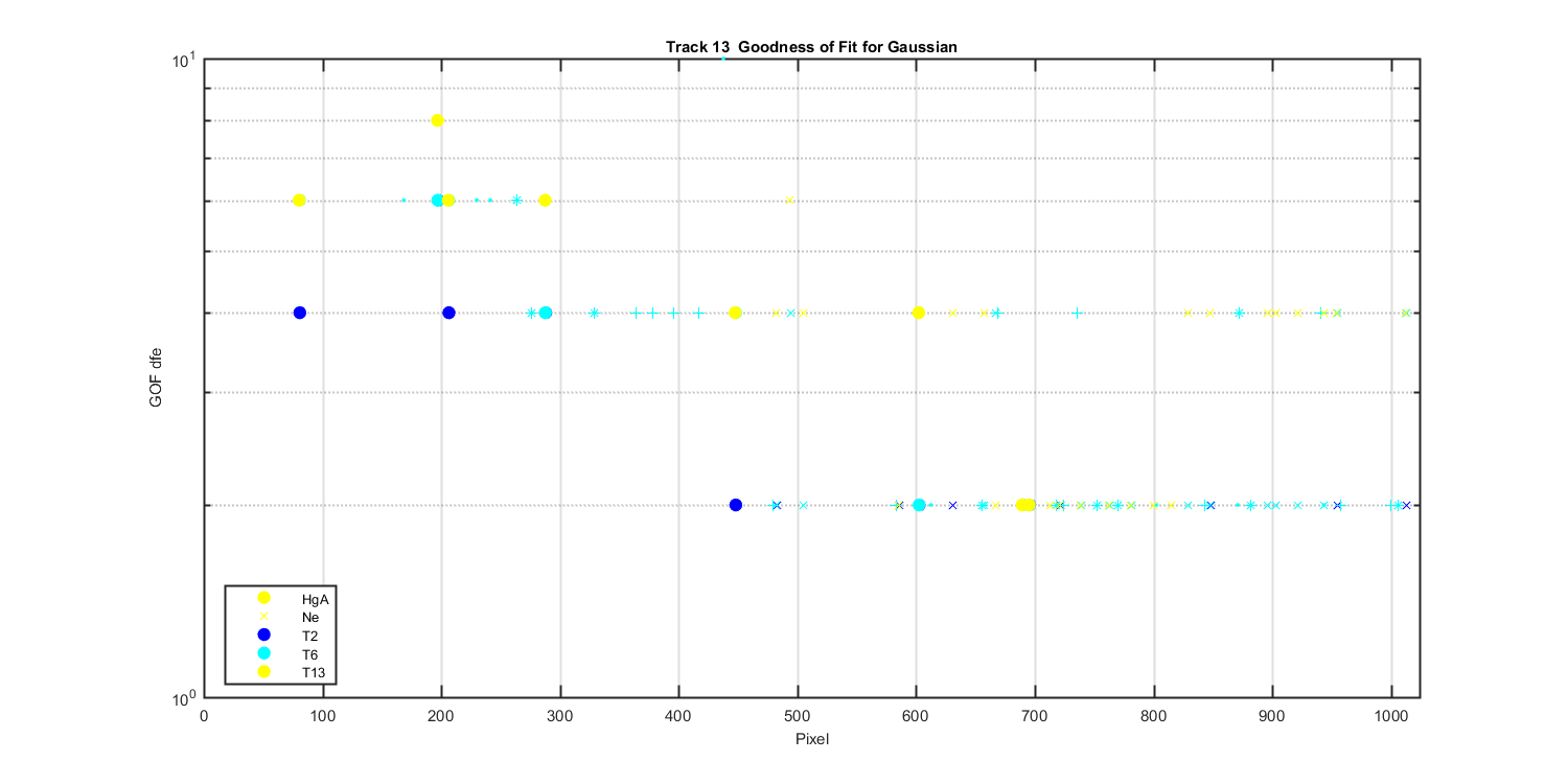
Figure 9
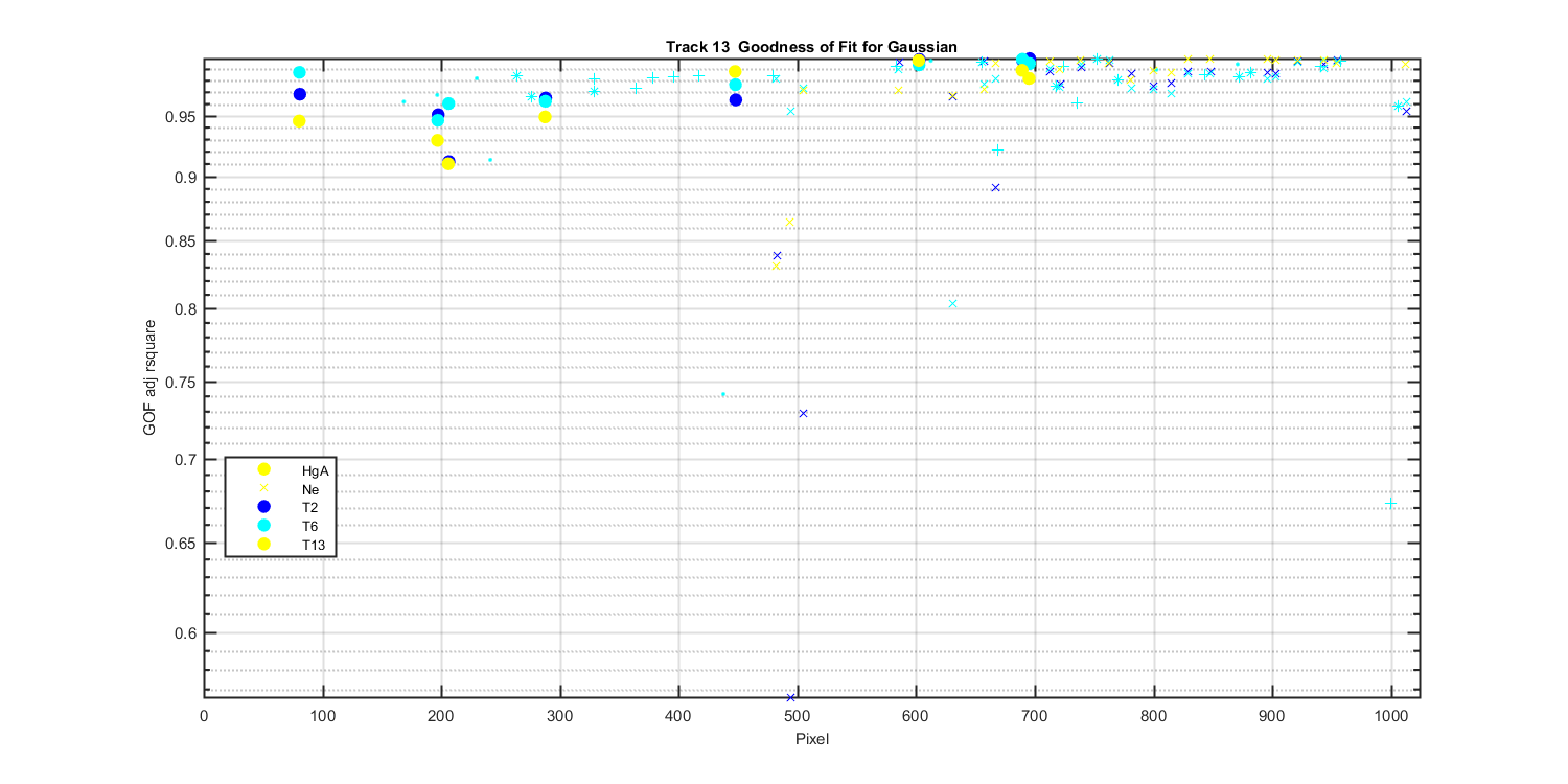
Figure 10
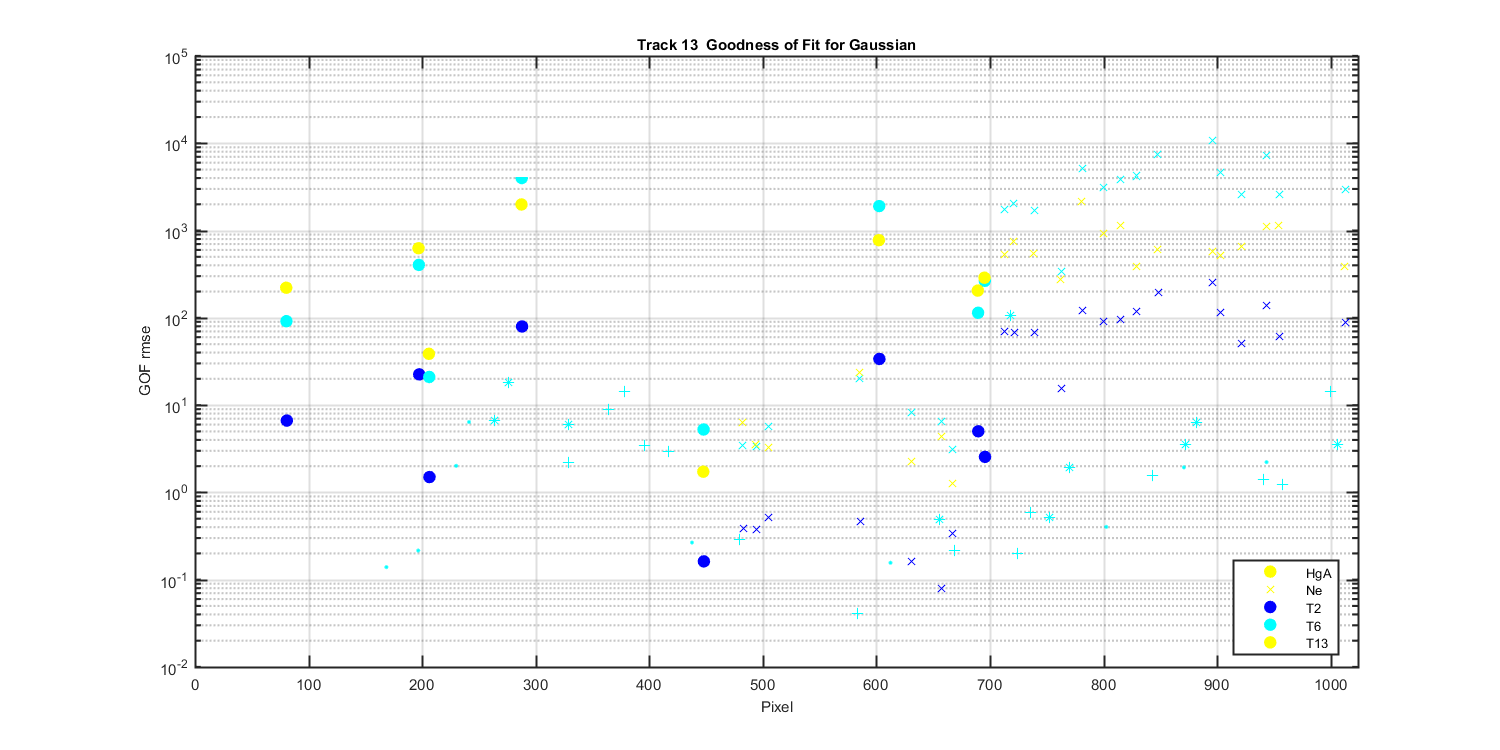
Figure 11