REVISION DATE: 31-Oct-2017 14:15:08

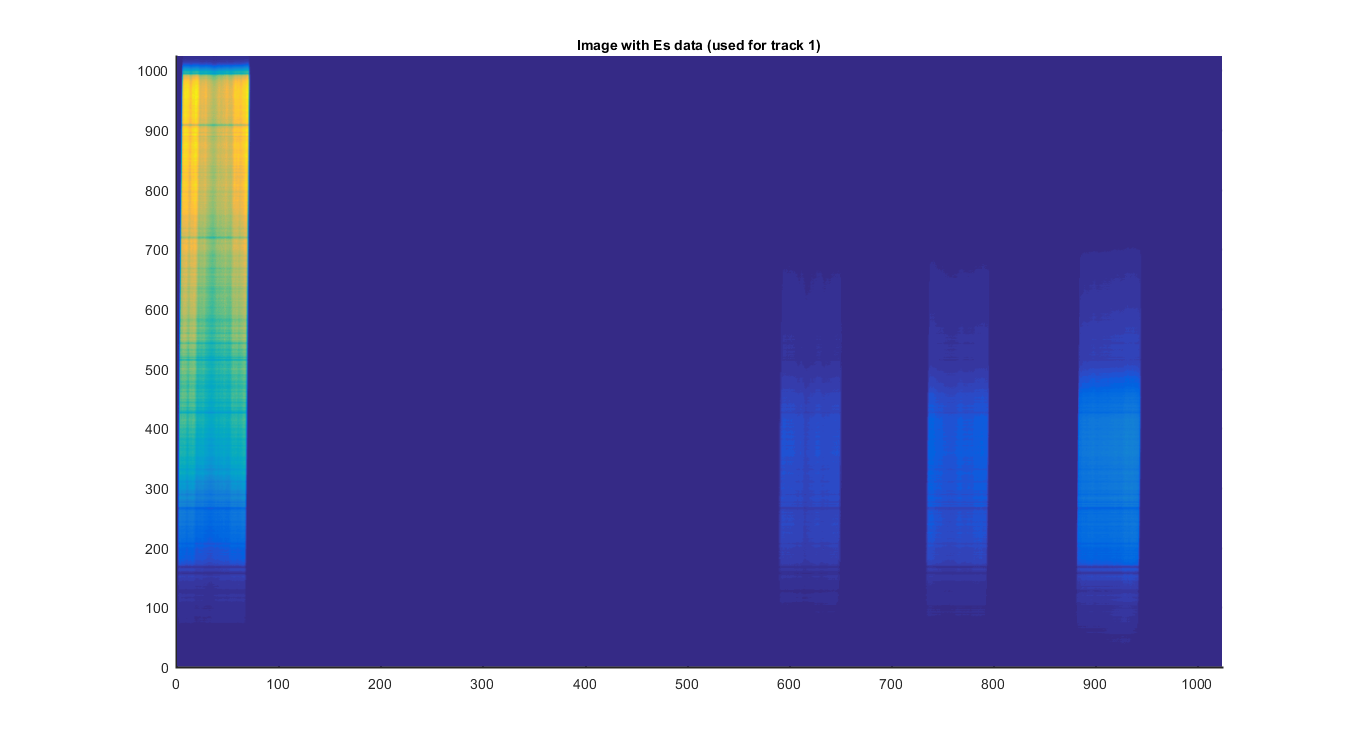
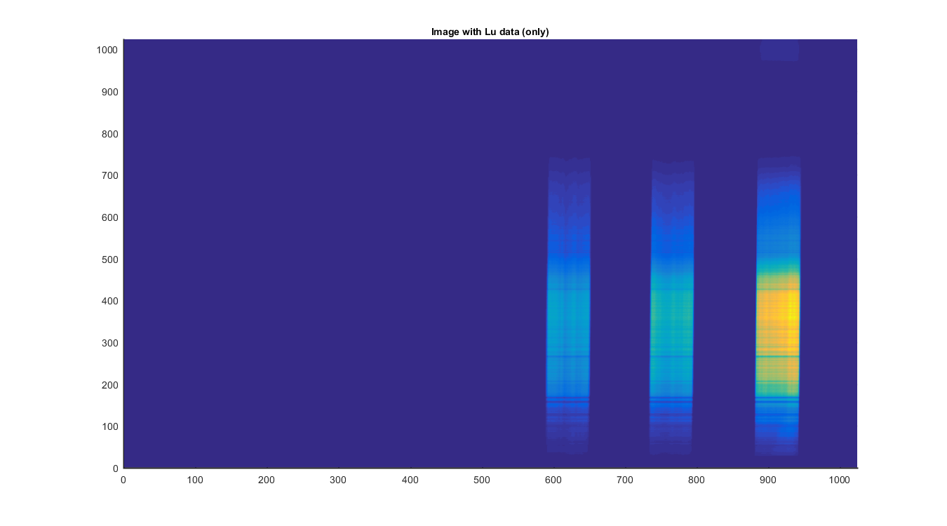
Kens Track width experiment. The idea of this experiment is to fine what the track width should be for a full track. I.E. how far out should the track width go? I used the day06 MOBY262 in-water data. For the Es track I used the only data set which has Es. For the Lus tracks I used the data set with Lu only (No Es). This way I got he highest levels for each track to do this experiment.

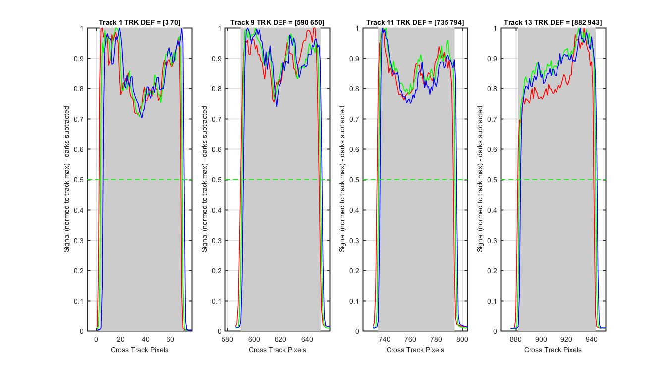
For each track I started with the track width at the pixel we found at the 50% line. See starting track definition below. I then added one pixel to each side of the track definitions until I had added 10 pixel (or increased the width by 20 pixels). The graphs are plotted spectrally for each track definition. I then took each track created and plotted a single vlues at 140, 360, 600 and 940 pixels verse (CPIX) the number of pixels added. So you could see the decrease in ADU for the different track defintions and different pixels aross the array. Finally I plotted the change in the ADU for each track definition and Cpic to see where the change was largest bases on pixels added. I did this for each track 1, 9, 11 and 13.

Starting track definitions.... TRACKS = [ 1 9 11 13];
LEDGE = [ 3 590 735 882];
REDGE = [70 650 794 943];

Image used for the Es track shifting fun. Obviously you can only add so many pixels to the left. So once the left side got to pixel 1 it just stayed there and the pixel width only increased by 1 and not 2 each time. The image is and average of 6 darks and 5 lite images. No division by int time or number of pixels averaged.

Figure 1

The image used for the 3 Lu Tracks. No Es data are collected on this data set so the Lu data have a higher ADU. The image is and average of 6 darks and 5 lite images. No division by int time or number of pixels averaged.

Figure 2

The starting track dfinitions for each track is in grey.

Figure 3

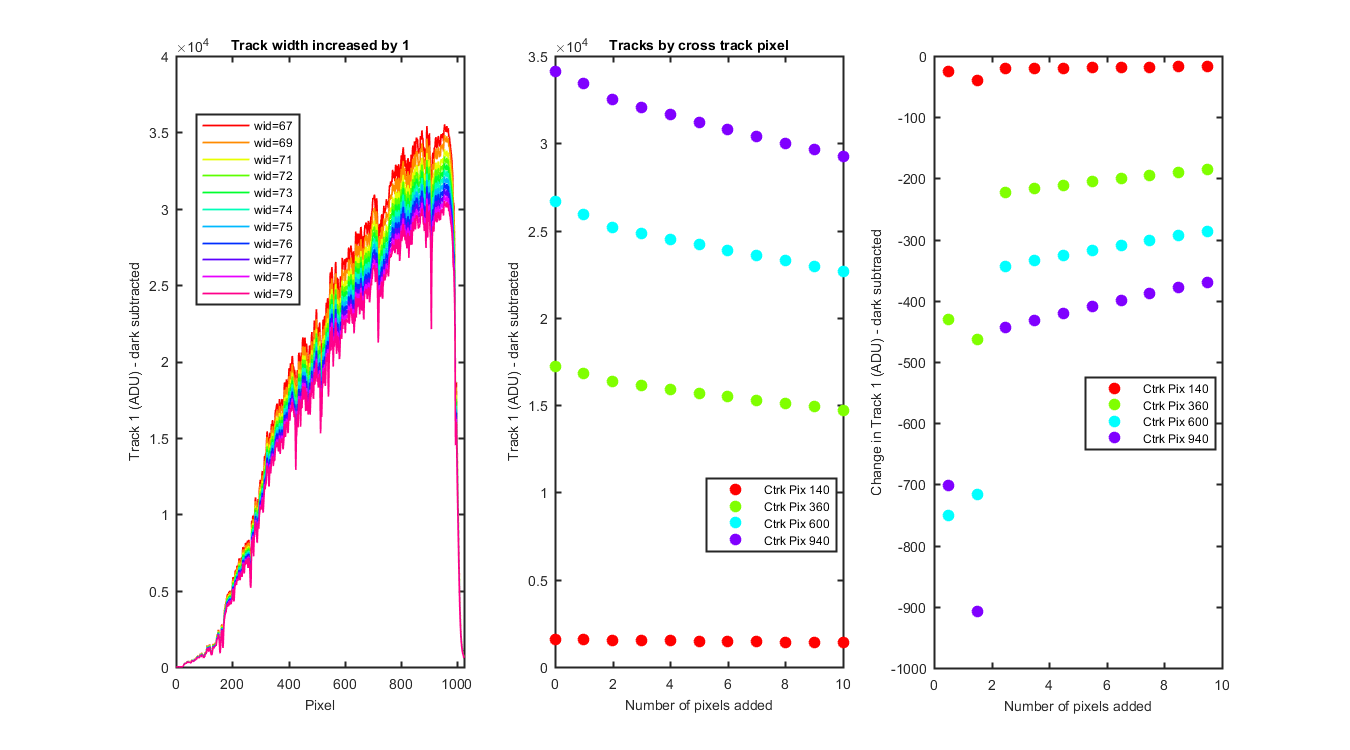
TRACK 1 ES DATA
Left panel is each track spectrally. Middle panel I took each track and plotted the value as pixel = cpix (see the color in the legend) verse the number of pixels added to each side of the track. The right panel is the same data as the middle but the difference is plotted to see where the large changes are.

Figure 4

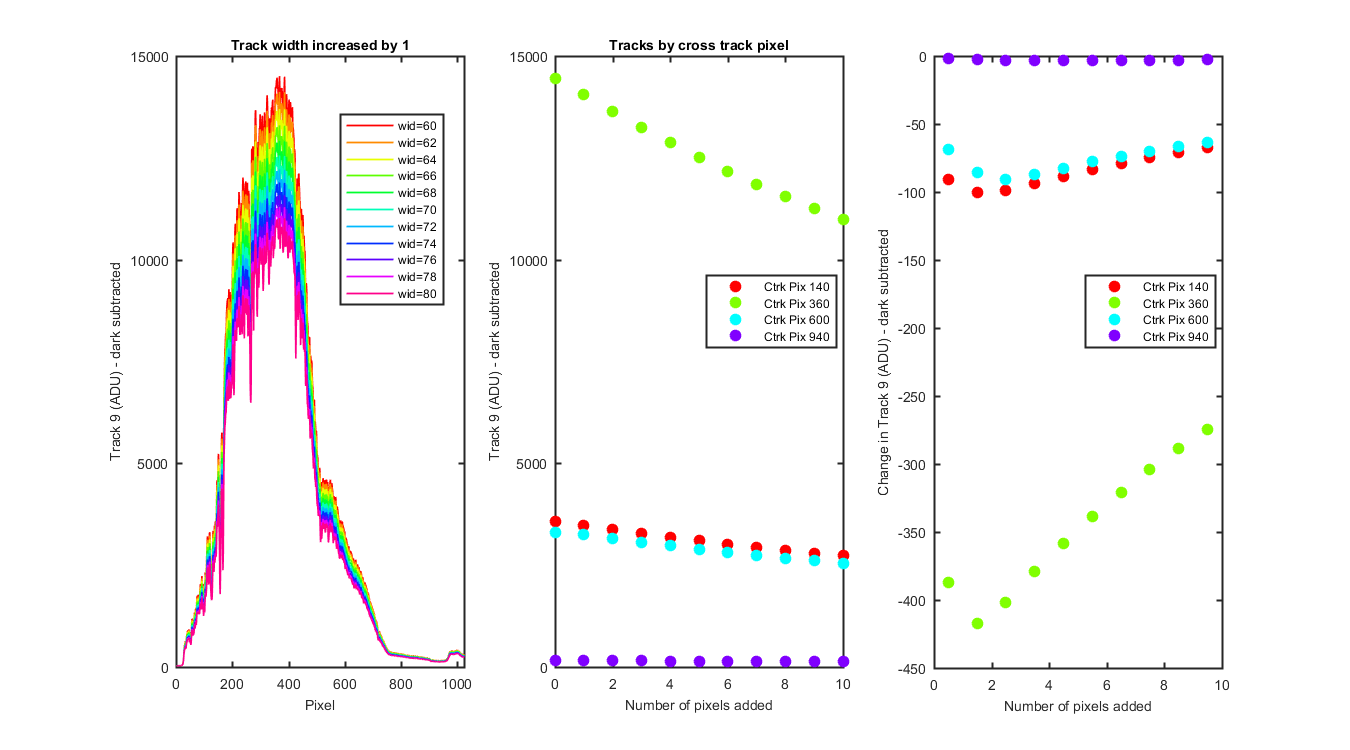
TRACK 9 LuTop DATA
Left panel is each track spectrally. Middle panel I took each track and plotted the value as pixel = cpix (see the color in the legend) verse the number of pixels added to each side of the track. The right panel is the same data as the middle but the difference is plotted to see where the large changes are.

Figure 5

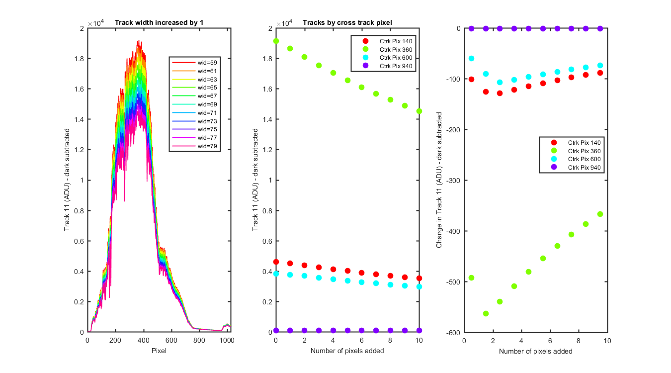
TRACK 11 LuMid DATA
Left panel is each track spectrally. Middle panel I took each track and plotted the value as pixel = cpix (see the color in the legend) verse the number of pixels added to each side of the track. The right panel is the same data as the middle but the difference is plotted to see where the large changes are.

Figure 6

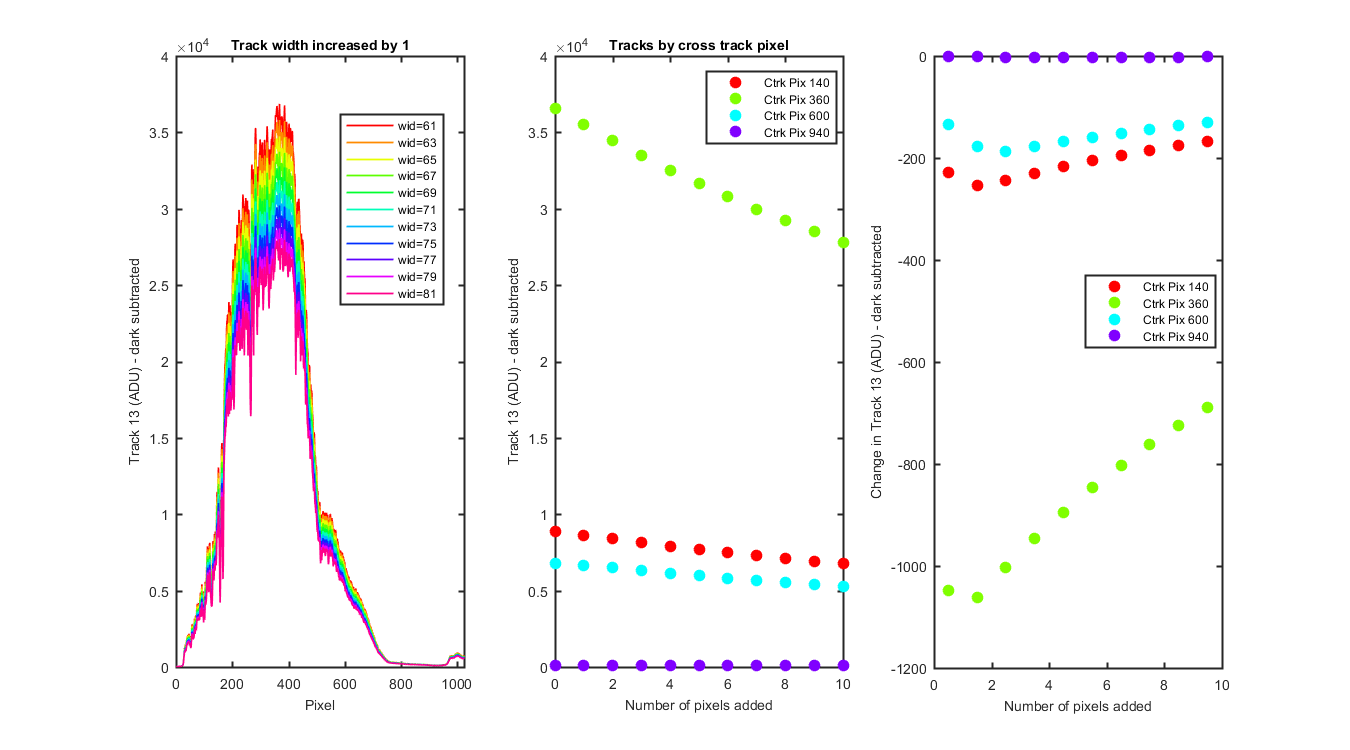
TRACK 13 LuBot DATA
Left panel is each track spectrally. Middle panel I took each track and plotted the value as pixel = cpix (see the color in the legend) verse the number of pixels added to each side of the track. The right panel is the same data as the middle but the difference is plotted to see where the large changes are.

Figure 7