REVISION DATE: 07-Dec-2015 17:02:33
Part of an Email from Casey Smith on 7/1/2015 3:15 PM:
The "sphere" cube has all of the channels illuminated.  "Channel 7" is only 7, obviously.  Helium red and helium blue show the same
helium discharge spectra at different integration levels in order to get data in the blue where the signal is weaker.

MIKES EMAIL ------------------
I looked at the NIST Atomic Spectra Database for Helium lines (in-air, nm)
( http://www.nist.gov/pml/data/asd.cfm,  "Lines",  "He I,   500 to 1000 nm"  )
Casey send four bip files (channel7.bip helium blue.bip helium red.bip sphere.bip).
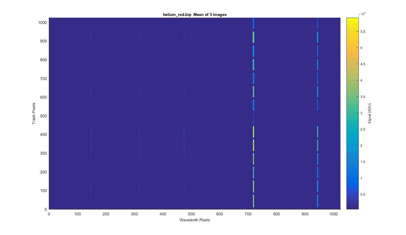
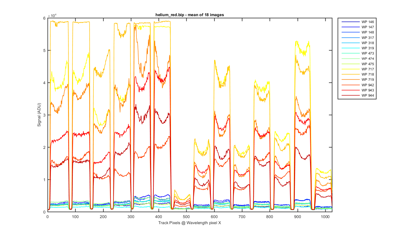
Below are my graphs of the helium red.bip. The file contains 3 images of the helium lamp source. This the red side is not saturated and the blue lines are usable too. See each graph below for more detail.
I took the 3 images and meaned them to get the surface plot below. For this file the red lines are not saturated and the blue lines are low but usable.
Figure 1
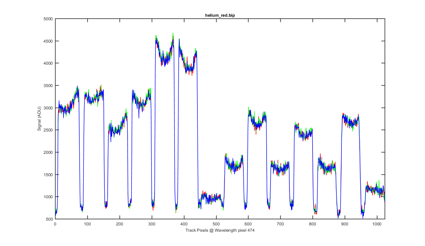
This is a cross section through the tracks at wavelength pixel 474, with one line for each of the 3 images. The tracks and their shapes look really stable.
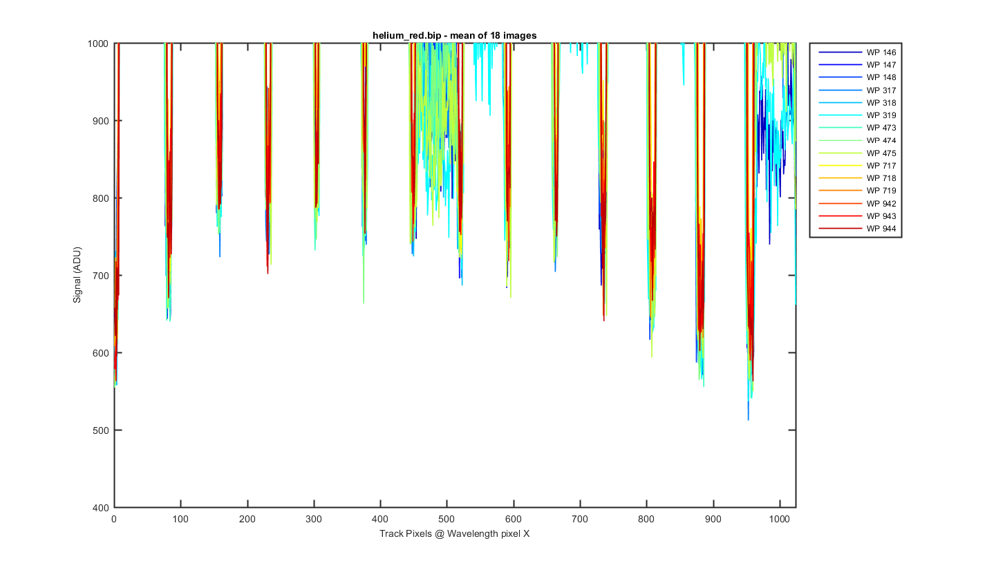
Figure 2
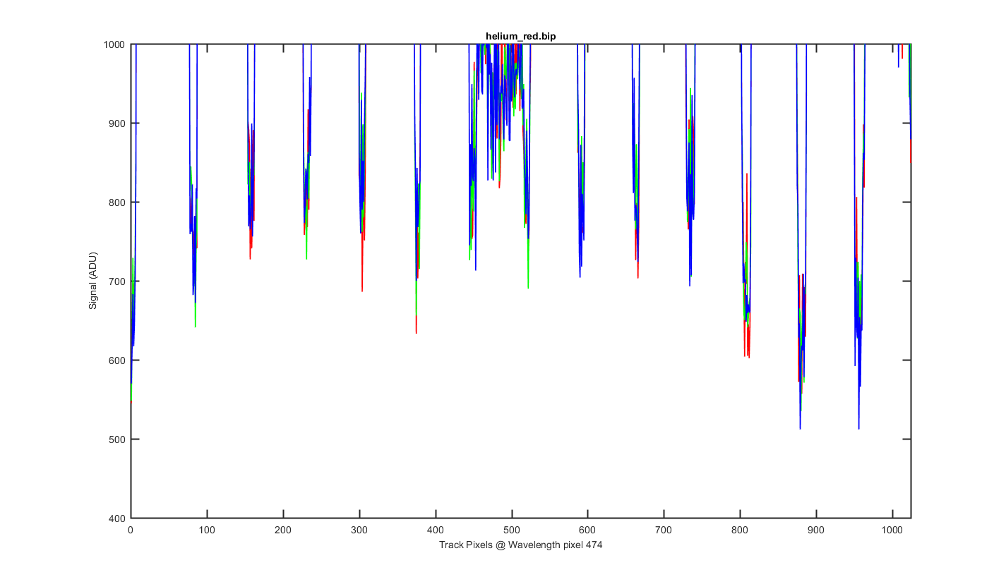
Same as the previous graph but zoomed into the bottom to see the level of the darks between the tracks.
Figure 3
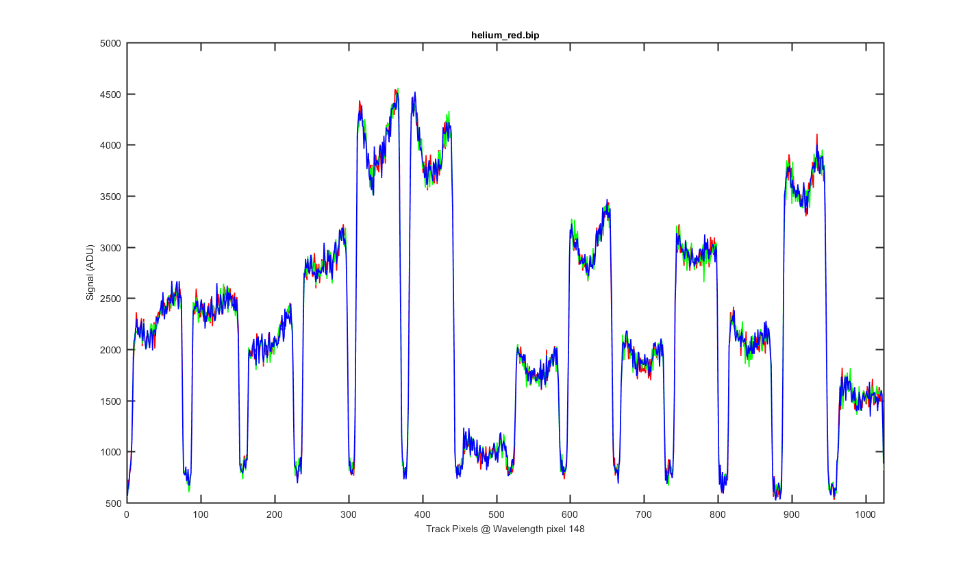
Same as figure 2 but for Wavelength pixel 148.
Figure 4
Again this is the mean image with slices thought the image at different wavelength pixels. The pixels choosen are where the helium peaks are and +- pixel pixel around them.
Figure 5
Same as figure 5 but zoomed to the bottom so you can see the darks between the tracks.
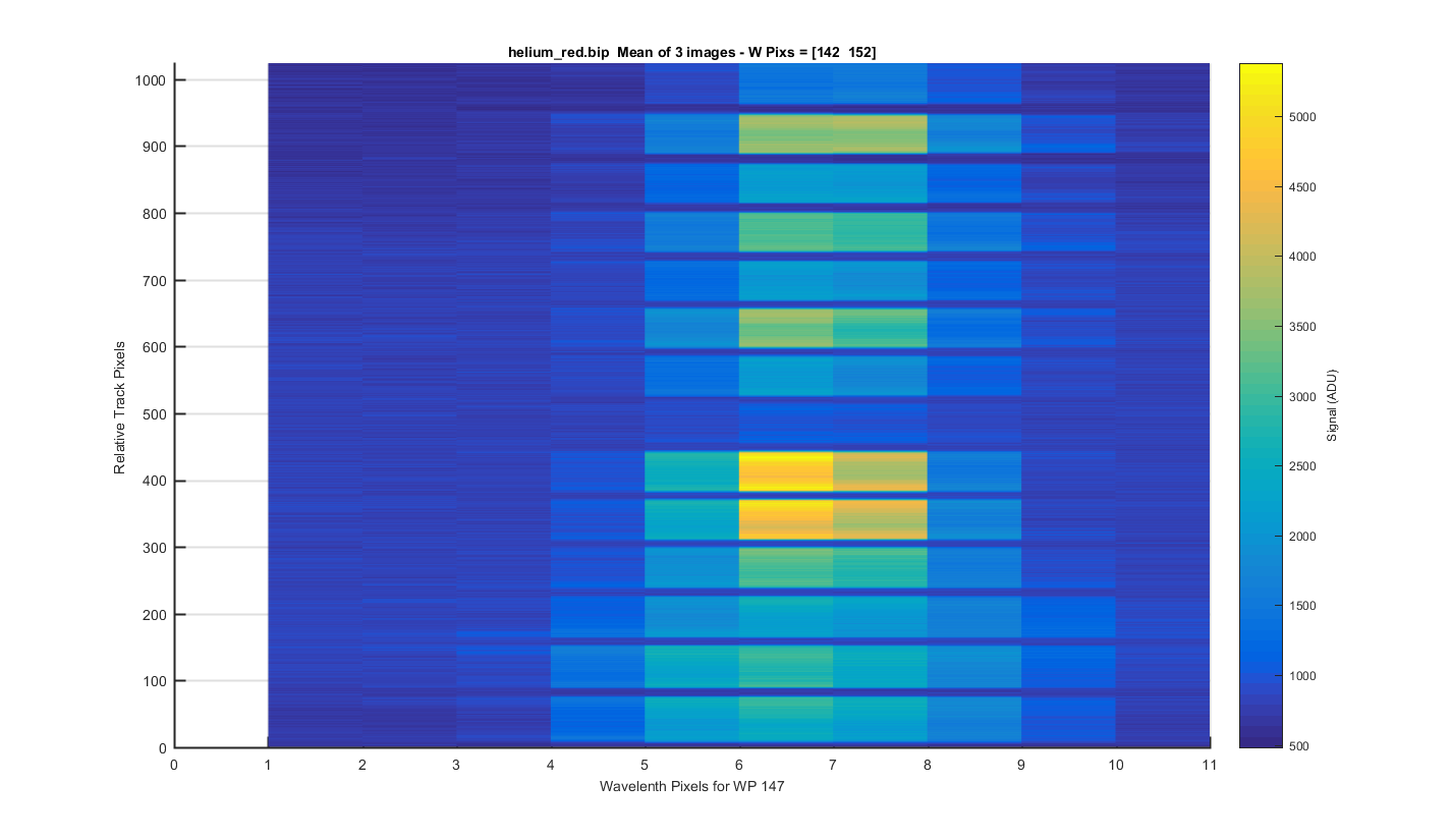
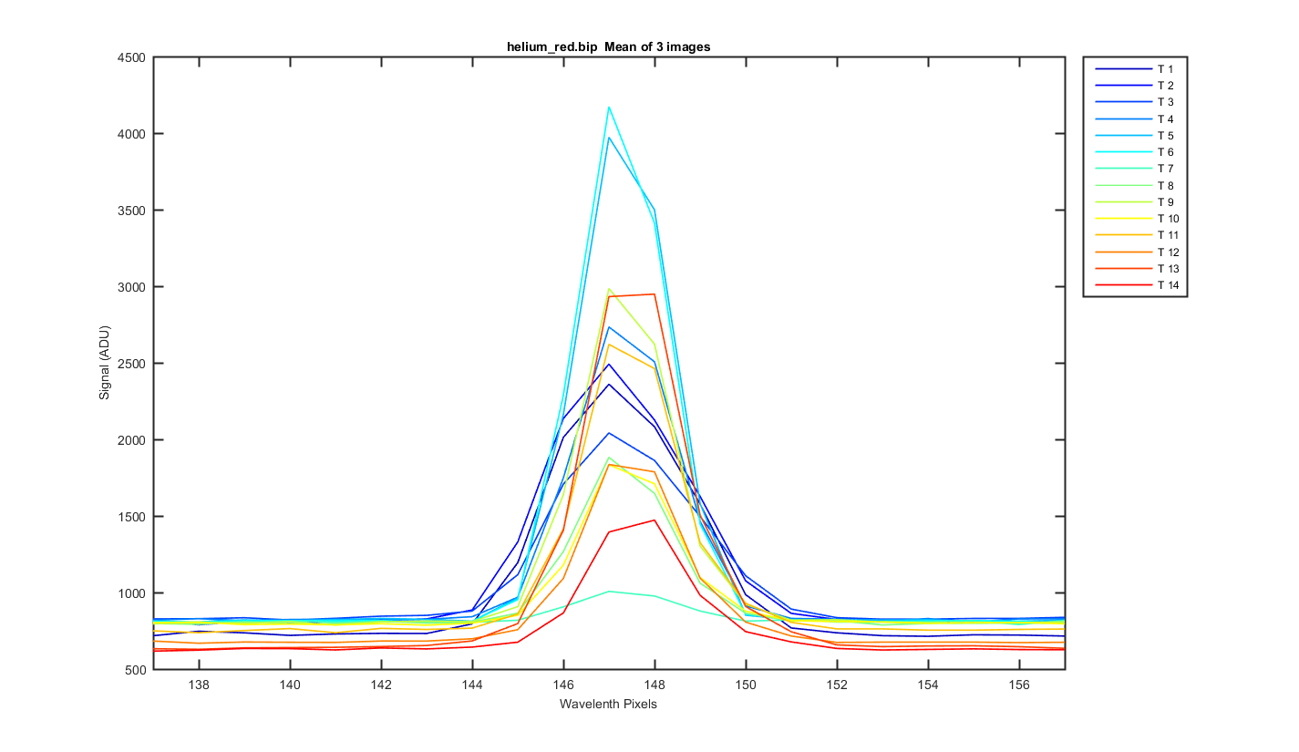
Figure 6
Helium Peak 1 (at pix 147): The same surface plot but showing how individual helium peaks line up from track to track. Looks pretty good!
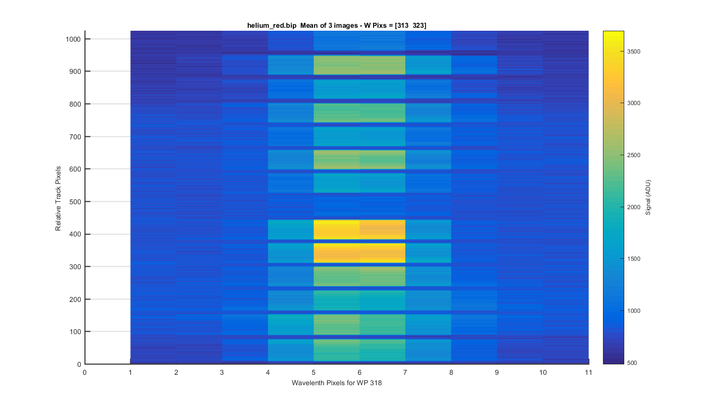
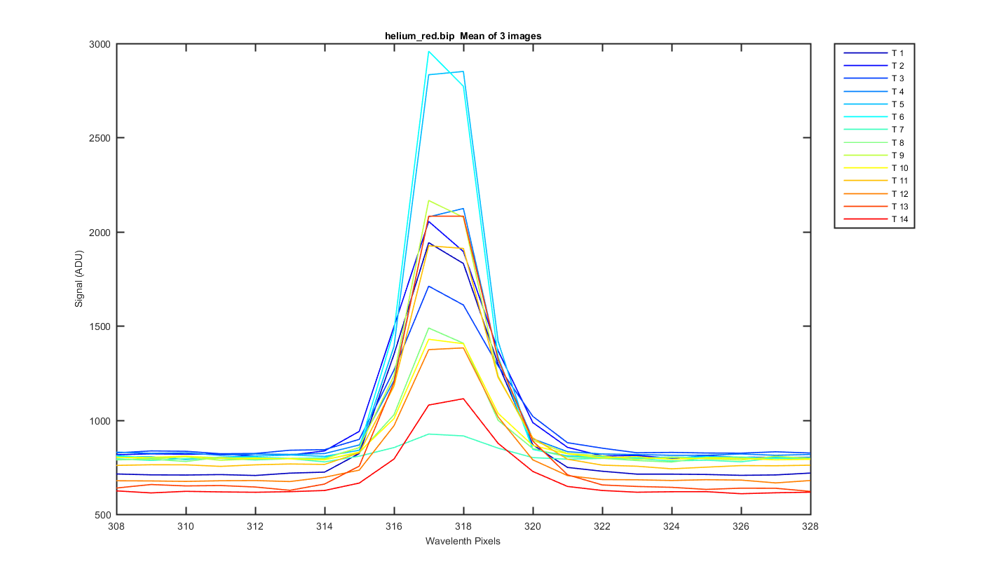
Figure 7
Helium Peak 2 (at pix 318): The same surface plot but showing how individual helium peaks line up from track to track. Looks pretty good!
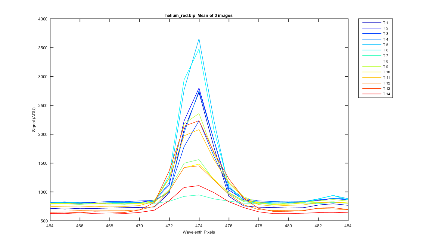
Figure 8
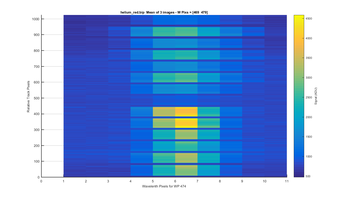
Helium Peak 3 (at pix 474): The same surface plot but showing how individual helium peaks line up from track to track. Looks pretty good!
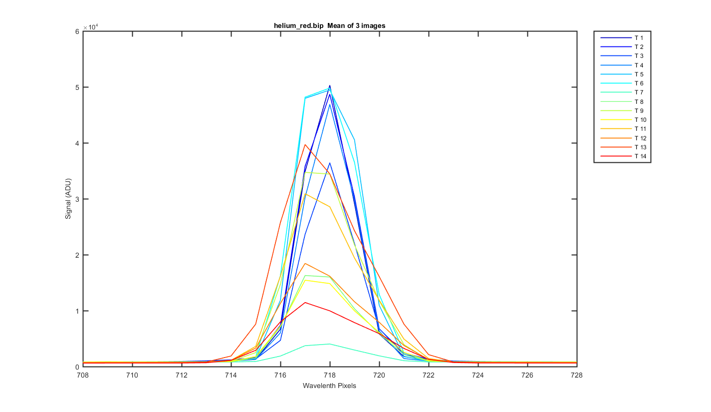
Figure 9
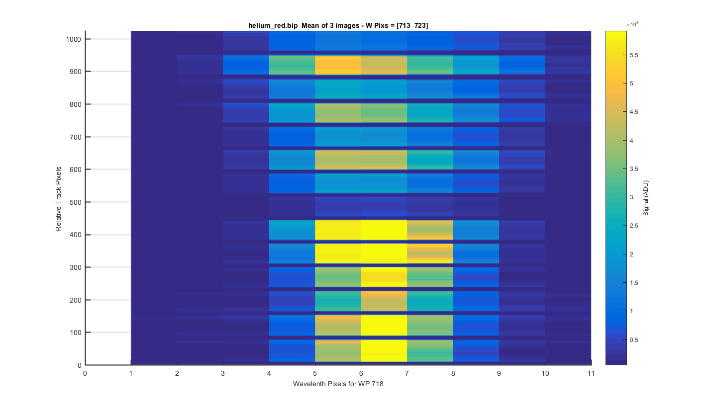
Helium Peak 4 (at pix 718): The same surface plot but showing how individual helium peaks line up from track to track. Looks pretty good!
Figure 10
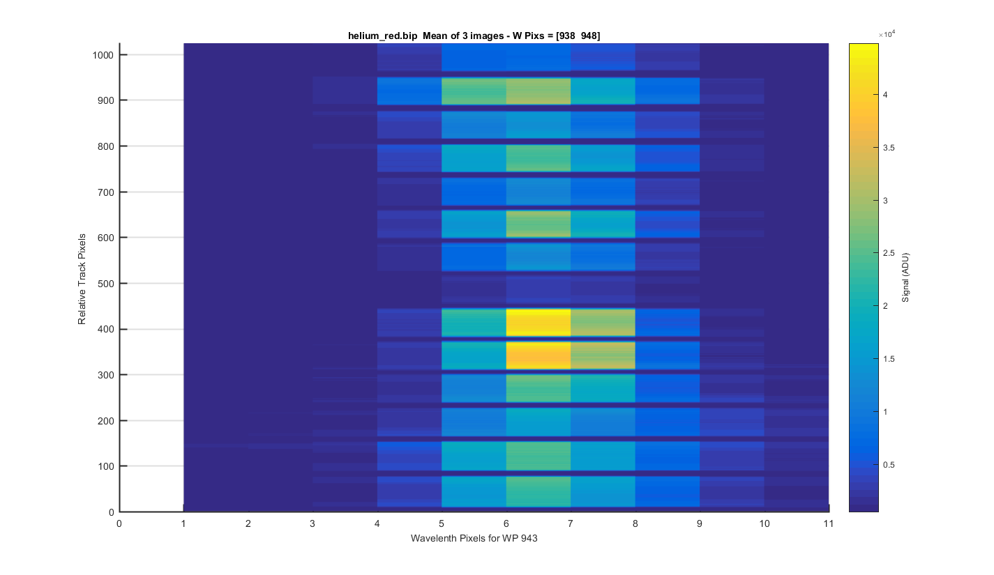
Helium Peak 5 (at pix 943): The same surface plot but showing how individual helium peaks line up from track to track. Looks pretty good!
Figure 11
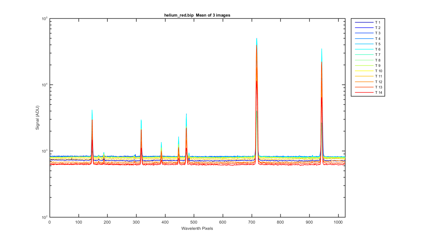
Mean image binned by track, the x-axis is wavelength pixels.
Figure 12
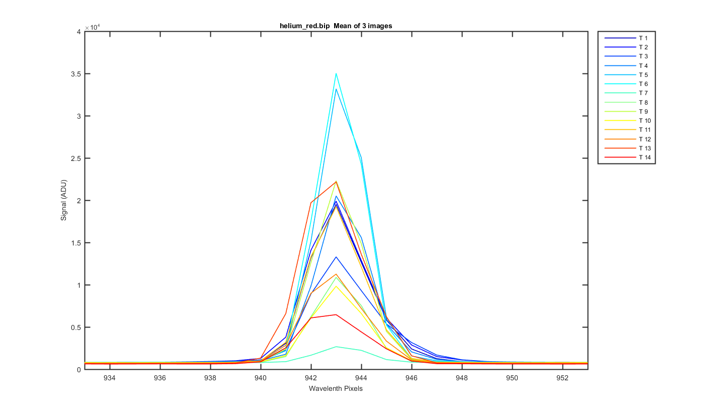
Close up of one of the helium peaks
Figure 13
Close up of one of the helium peaks
Figure 14
Close up of one of the helium peaks
Figure 15
Close up of one of the helium peaks
Figure 16
Close up of one of the helium peaks
Figure 17
MY VERY ROUGH GUESS AT A WAVELENGTH CAL!!! THIS ASSUMES I GUESS CORRECTLY WHICH PEAKS WHERE WHICH HELIUM LINES.
Track, Min,    Max,     diff
    1, 336.52, 695.39,  0.35
    2, 336.53, 695.41,  0.35
    3, 336.48, 695.40,  0.35
    4, 336.53, 695.32,  0.35
    5, 336.54, 695.33,  0.35
    6, 336.48, 695.39,  0.35
    7, 336.49, 695.43,  0.35
    8, 336.52, 695.39,  0.35
    9, 336.50, 695.40,  0.35
   10, 336.49, 695.41,  0.35
   11, 336.46, 695.46,  0.35
   12, 336.48, 695.46,  0.35
   13, 336.44, 695.51,  0.35
   14, 336.45, 695.45,  0.35
Figure 18
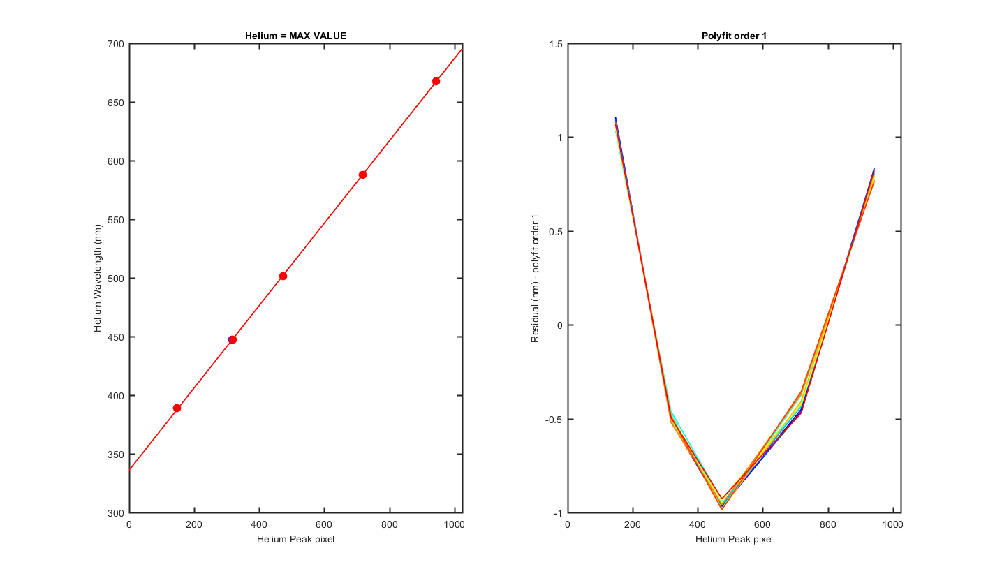
  Track = The Resonon Track number
Lwave = Laser Wavelength
Lpix1 = Laser Pixel found using the max value of the track
Lpix2 = Laser Pixel found using mygaussfit to fit the laser peak
| Track | Lwave | Lpix1 | Lpix2 |
|---|---|---|---|
| 1 | 388.8648 | 147 | 147.07 |
| 1 | 447.148 | 317 | 317.83 |
| 1 | 501.5678 | 474 | 474.26 |
| 1 | 587.5621 | 718 | 717.90 |
| 1 | 667.8151 | 943 | 943.01 |
| 2 | 388.8648 | 147 | 147.11 |
| 2 | 447.148 | 317 | 317.70 |
| 2 | 501.5678 | 474 | 474.22 |
| 2 | 587.5621 | 718 | 717.89 |
| 2 | 667.8151 | 943 | 942.96 |
| 3 | 388.8648 | 147 | 147.18 |
| 3 | 447.148 | 317 | 317.86 |
| 3 | 501.5678 | 474 | 474.26 |
| 3 | 587.5621 | 718 | 717.96 |
| 3 | 667.8151 | 943 | 942.98 |
| 4 | 388.8648 | 147 | 147.15 |
| 4 | 447.148 | 318 | 317.78 |
| 4 | 501.5678 | 474 | 474.30 |
| 4 | 587.5621 | 718 | 717.99 |
| 4 | 667.8151 | 943 | 943.27 |
| 5 | 388.8648 | 147 | 147.14 |
| 5 | 447.148 | 318 | 317.79 |
| 5 | 501.5678 | 474 | 474.26 |
| 5 | 587.5621 | 718 | 717.96 |
| 5 | 667.8151 | 943 | 943.24 |
| 6 | 388.8648 | 147 | 147.37 |
| 6 | 447.148 | 317 | 317.75 |
| 6 | 501.5678 | 474 | 474.22 |
| 6 | 587.5621 | 718 | 717.89 |
| 6 | 667.8151 | 943 | 943.15 |
| 7 | 388.8648 | 147 | 147.26 |
| 7 | 447.148 | 317 | 317.74 |
| 7 | 501.5678 | 474 | 474.27 |
| 7 | 587.5621 | 718 | 717.65 |
| 7 | 667.8151 | 943 | 943.10 |
| 8 | 388.8648 | 147 | 147.15 |
| 8 | 447.148 | 317 | 317.83 |
| 8 | 501.5678 | 474 | 474.14 |
| 8 | 587.5621 | 717 | 717.82 |
| 8 | 667.8151 | 943 | 943.12 |
| 9 | 388.8648 | 147 | 147.20 |
| 9 | 447.148 | 317 | 317.83 |
| 9 | 501.5678 | 474 | 474.22 |
| 9 | 587.5621 | 717 | 717.81 |
| 9 | 667.8151 | 943 | 943.10 |
| 10 | 388.8648 | 147 | 147.27 |
| 10 | 447.148 | 317 | 317.78 |
| 10 | 501.5678 | 474 | 474.15 |
| 10 | 587.5621 | 717 | 717.81 |
| 10 | 667.8151 | 943 | 943.08 |
| 11 | 388.8648 | 147 | 147.28 |
| 11 | 447.148 | 317 | 317.80 |
| 11 | 501.5678 | 474 | 474.29 |
| 11 | 587.5621 | 717 | 717.71 |
| 11 | 667.8151 | 943 | 942.95 |
| 12 | 388.8648 | 147 | 147.22 |
| 12 | 447.148 | 318 | 317.86 |
| 12 | 501.5678 | 474 | 474.19 |
| 12 | 587.5621 | 717 | 717.56 |
| 12 | 667.8151 | 943 | 943.02 |
| 13 | 388.8648 | 148 | 147.31 |
| 13 | 447.148 | 318 | 317.80 |
| 13 | 501.5678 | 474 | 474.26 |
| 13 | 587.5621 | 717 | 717.47 |
| 13 | 667.8151 | 943 | 942.92 |
| 14 | 388.8648 | 148 | 147.31 |
| 14 | 447.148 | 318 | 317.85 |
| 14 | 501.5678 | 474 | 474.16 |
| 14 | 587.5621 | 717 | 717.91 |
| 14 | 667.8151 | 943 | 942.91 |