REVISION DATE: 17-Oct-2019 14:10:37
The Heilum wave cal data.
Below are my graphs of the helium data. The file contains 10 images of the helium lamp source. All the data are dark subtracted. See each graph below for more detail.
Track Wavelength fits:
P(1,:) = [-6.384111e-09  2.155553e-05     0.3337342      339.4072]
P(2,:) = [-6.880806e-09   2.25018e-05     0.3332042      339.4771]
P(3,:) = [-6.713687e-09  2.228478e-05     0.3332468      339.4855]
P(4,:) = [-6.105725e-09  2.134033e-05     0.3336215      339.4531]
P(5,:) = [-6.131641e-09  2.136169e-05     0.3336244      339.4457]
P(6,:) = [-6.22549e-09  2.143707e-05     0.3336624      339.4462]
P(7,:) = [-6.451137e-09  2.172488e-05     0.3335982      339.4441]
P(8,:) = [-6.08166e-09  2.126004e-05      0.333735       339.404]
P(9,:) = [-6.422372e-09  2.171143e-05     0.3336244      339.3882]
P(10,:) = [-6.422535e-09   2.16989e-05     0.3336703      339.3653]
P(11,:) = [-6.282548e-09  2.152884e-05     0.3337542      339.3183]
P(12,:) = [-6.536746e-09  2.188308e-05     0.3336852      339.2973]
P(13,:) = [-6.49664e-09  2.185956e-05     0.3337058      339.2693]
P(14,:) = [-6.360985e-09  2.178533e-05     0.3336566      339.2802]
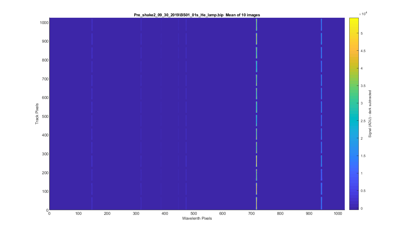
Figure 1 Resonon took dark scans for the two int times taken. So I meaned all the dark images for the 1s data and subtracted it from the data before processing. I Then took the 10 images and meaned them to get the surface plot below.
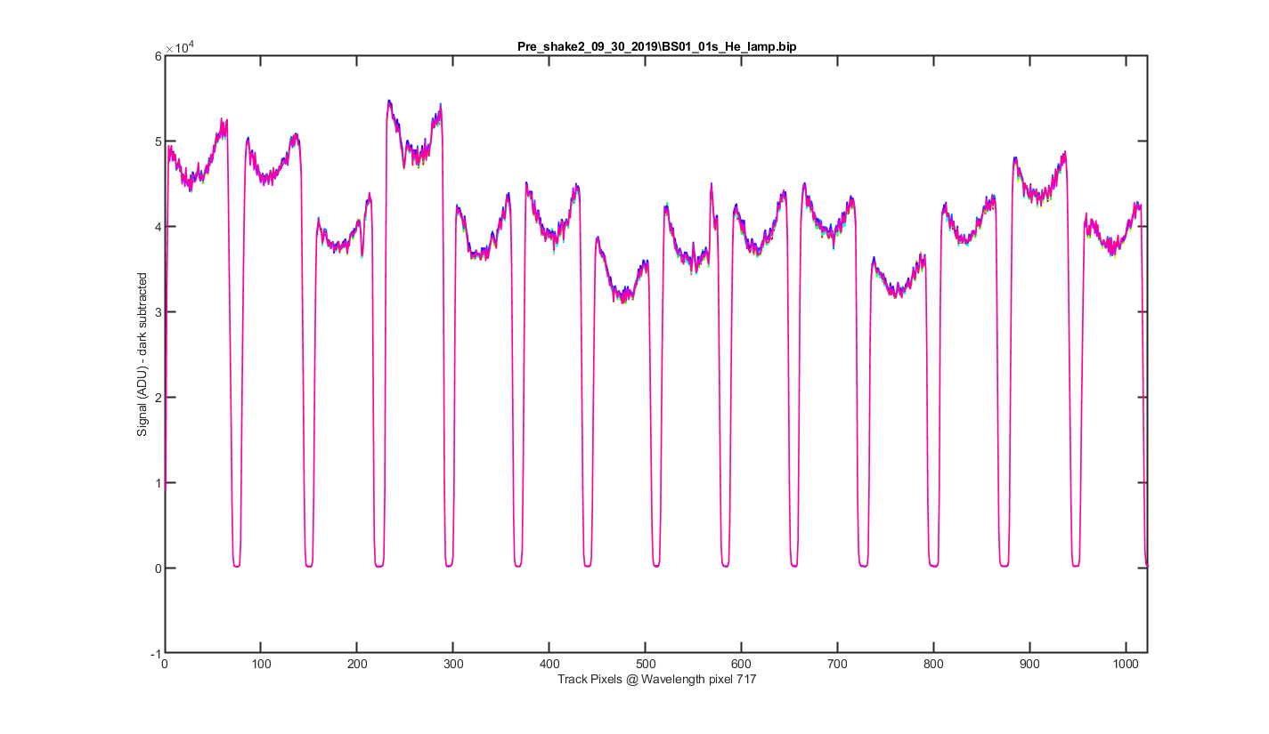
Figure 2 This is a cross section through the tracks at wavelength pixel 694, with one line for each of the 10 images. The tracks and their shapes look really stable.
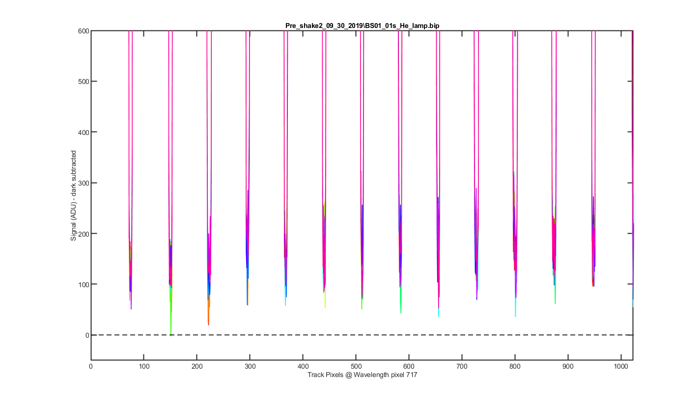
Figure 3 Same as the previous graph but zoomed into the bottom to see the level of the darks between the tracks.
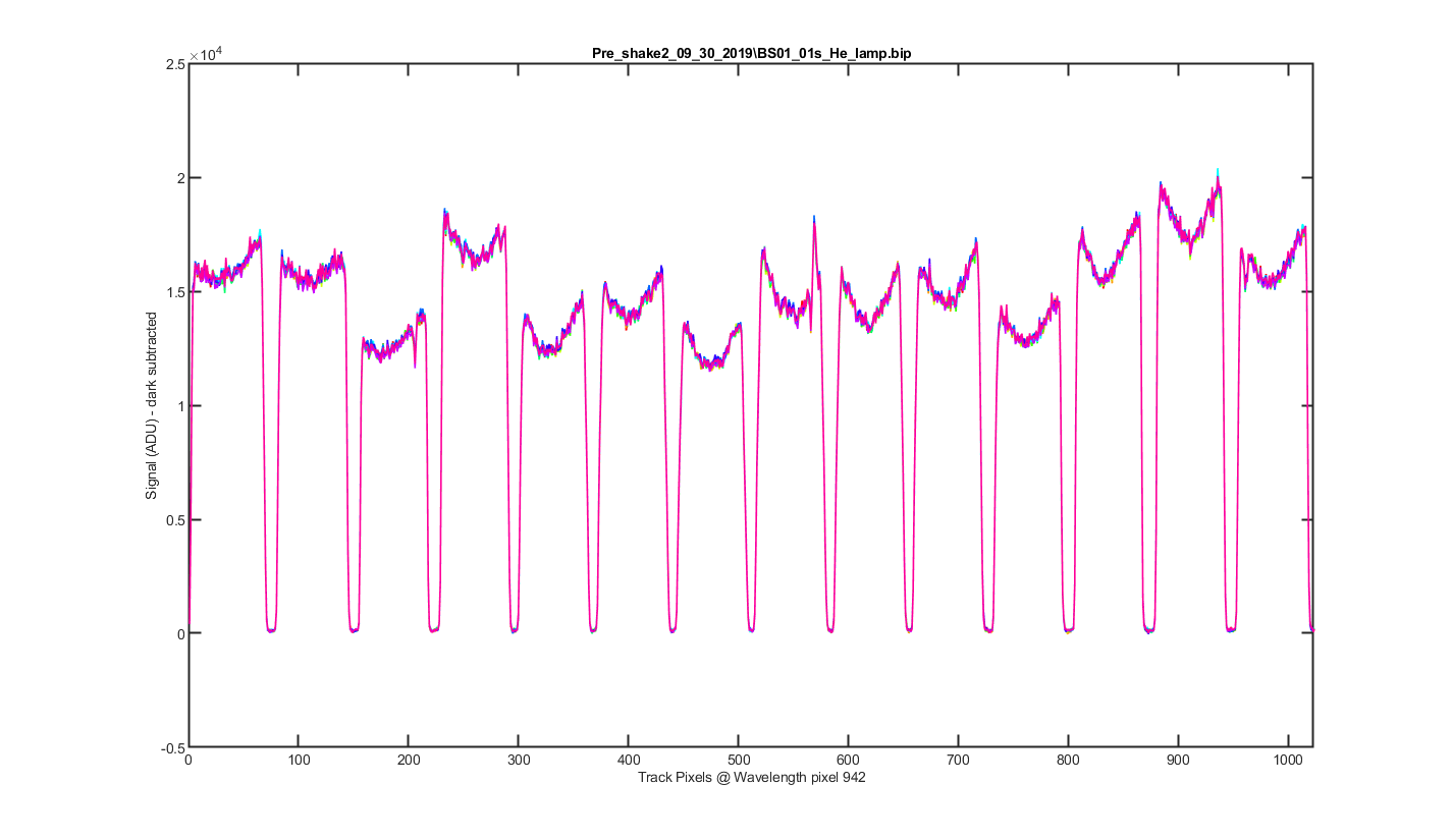
Figure 4 Same as figure 2 but for Wavelength pixel 920.
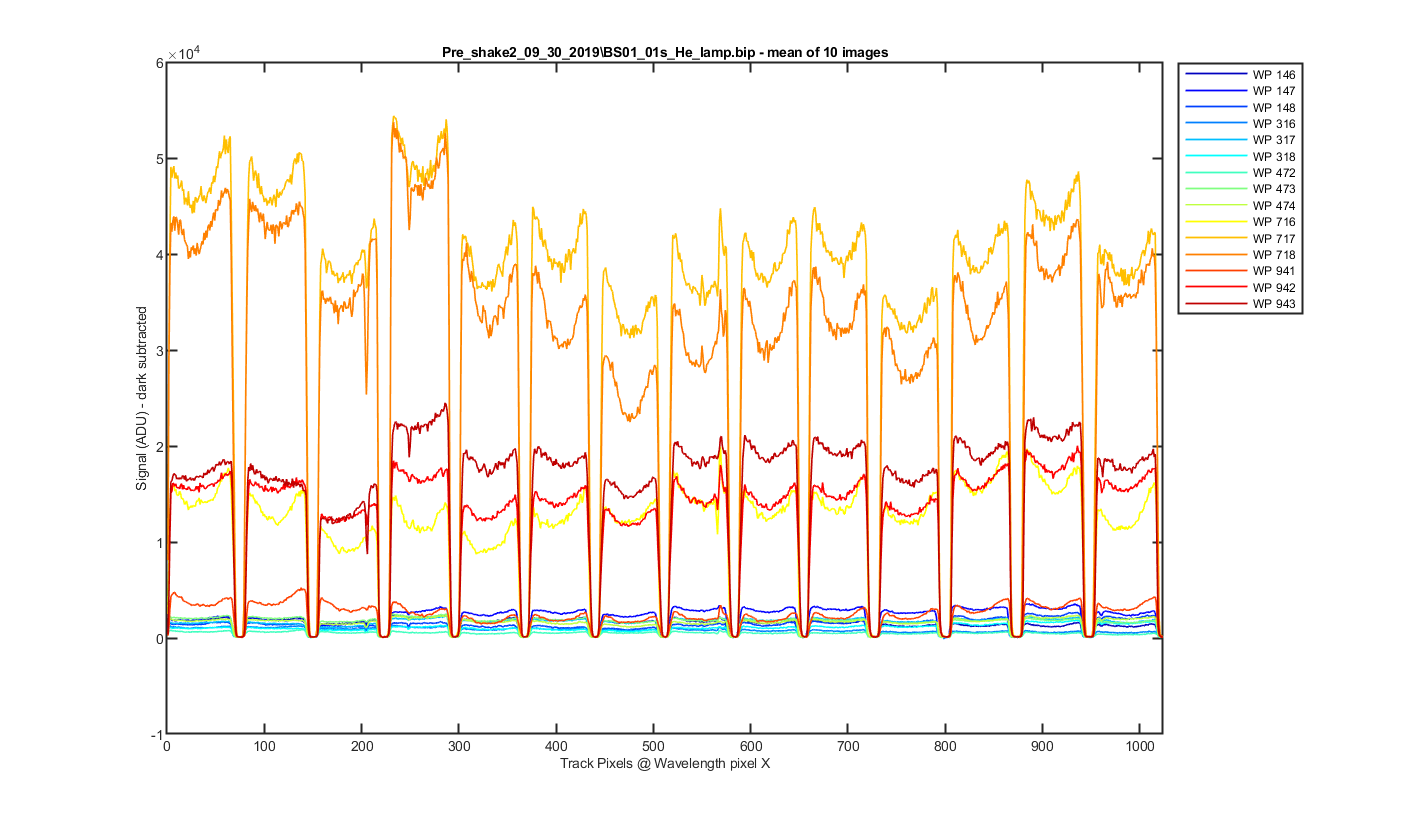
Figure 5 Again this is the mean image with slices thought the image at different wavelength pixels. The pixels choosen are where the helium peaks are and +- pixel pixel around them.
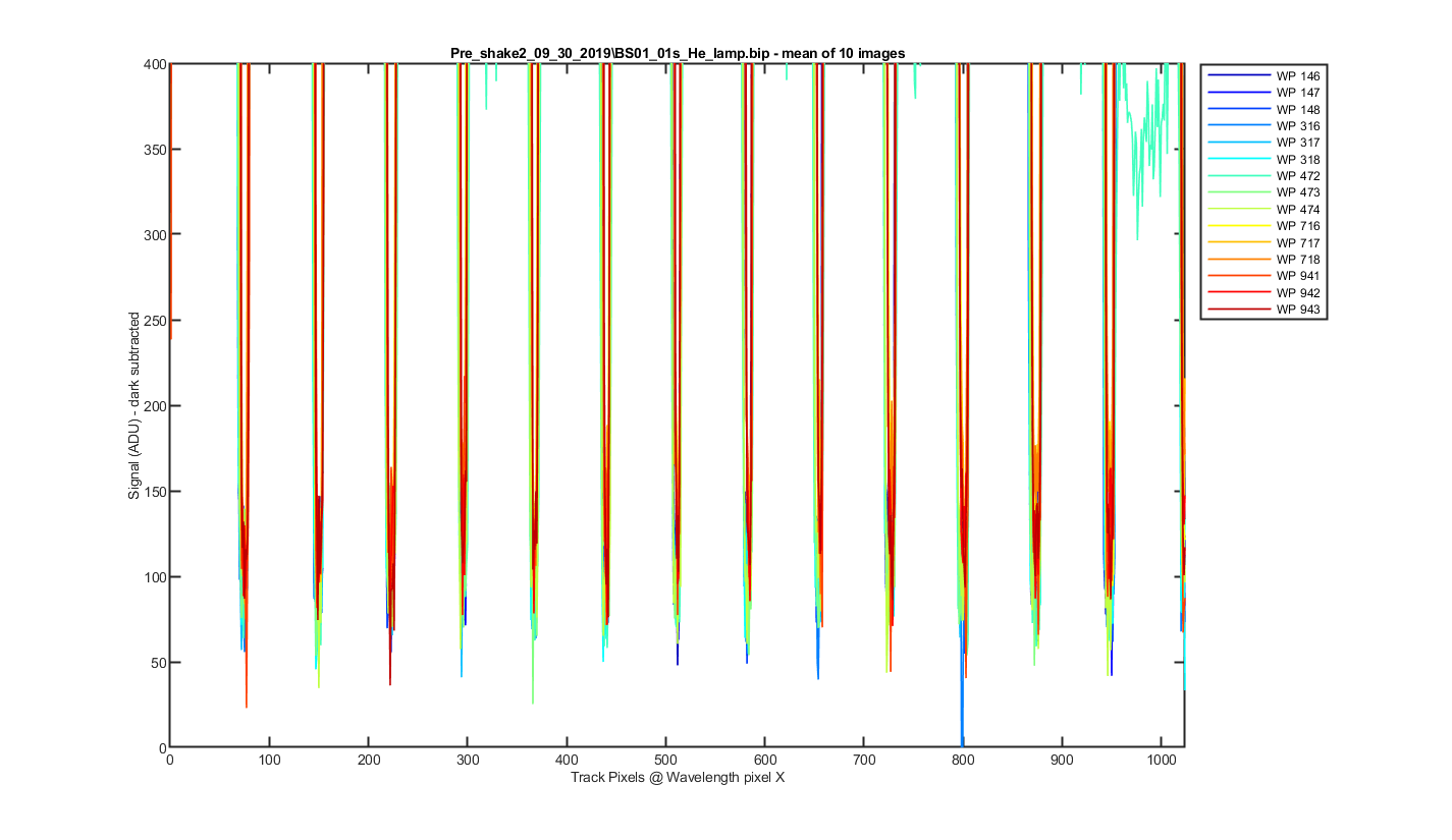
Figure 6 Same as figure 5 but zoomed to the bottom so you can see the darks between the tracks.
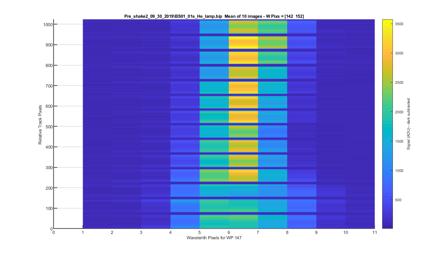
Figure 7 Helium Peak 1 (at pix 147): The same surface plot but showing how individual helium peaks line up from track to track.
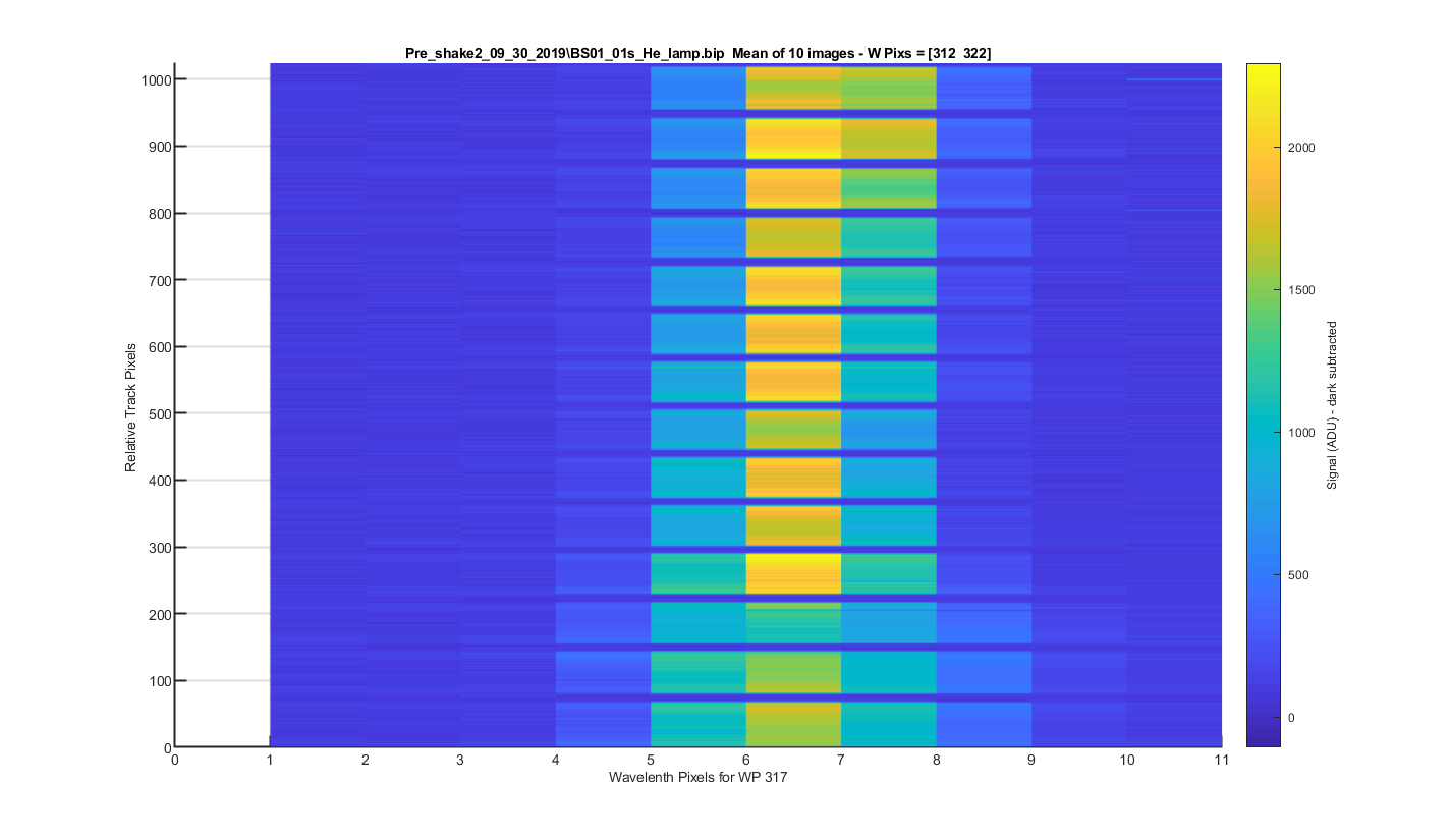
Figure 8 Helium Peak 2 (at pix 317): The same surface plot but showing how individual helium peaks line up from track to track.
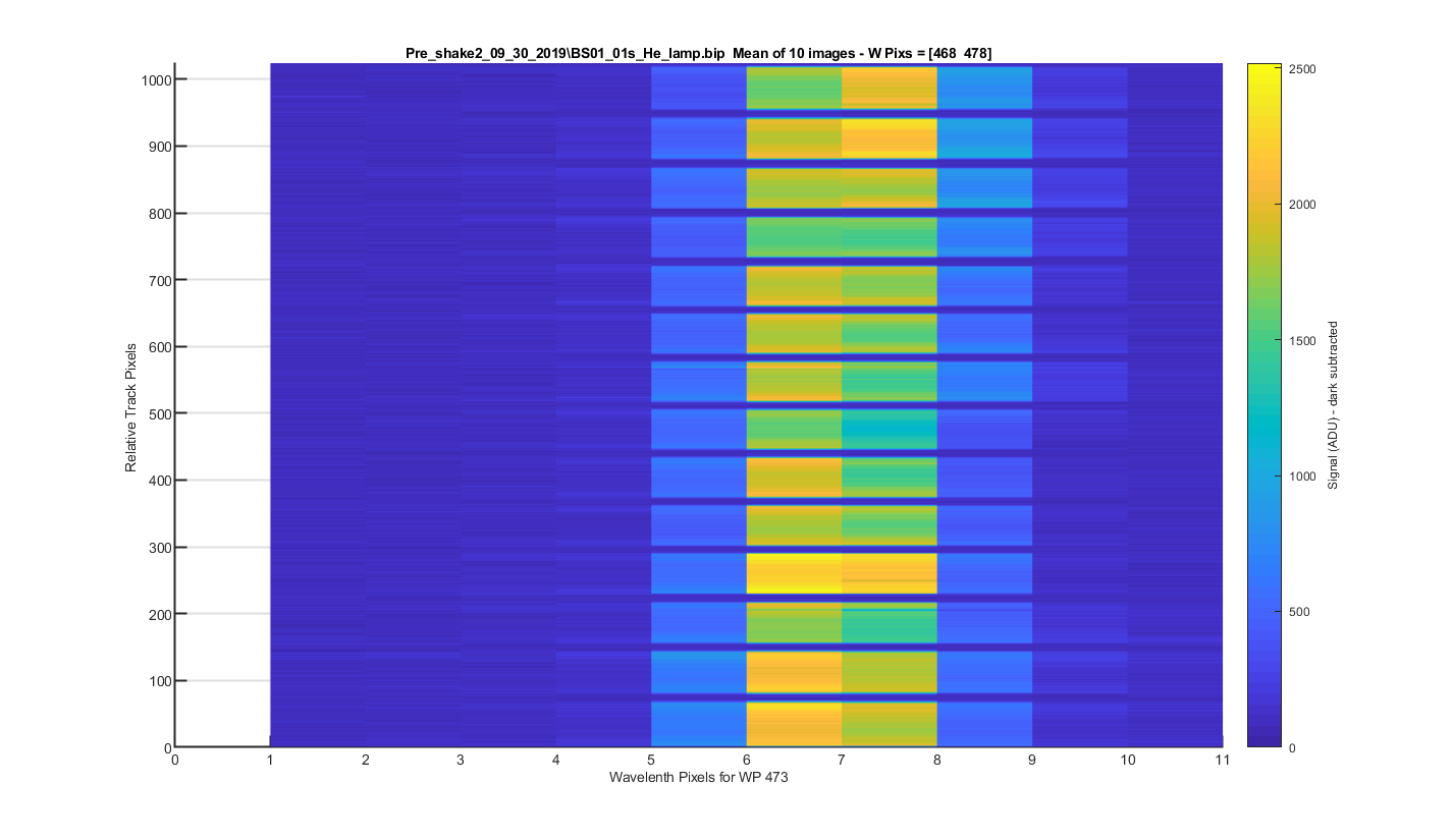
Figure 9 Helium Peak 3 (at pix 473): The same surface plot but showing how individual helium peaks line up from track to track.
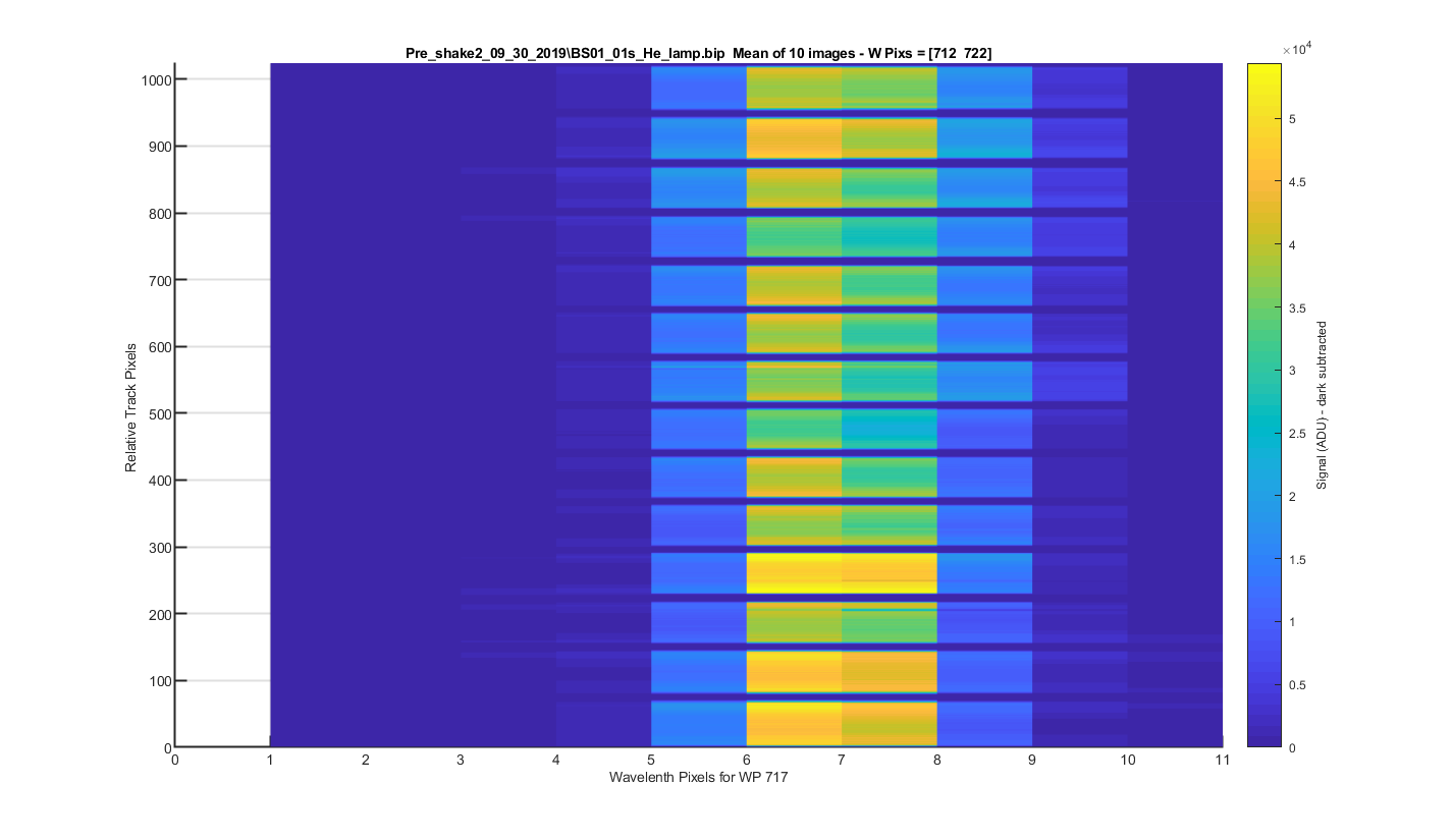
Figure 10 Helium Peak 4 (at pix 717): The same surface plot but showing how individual helium peaks line up from track to track.
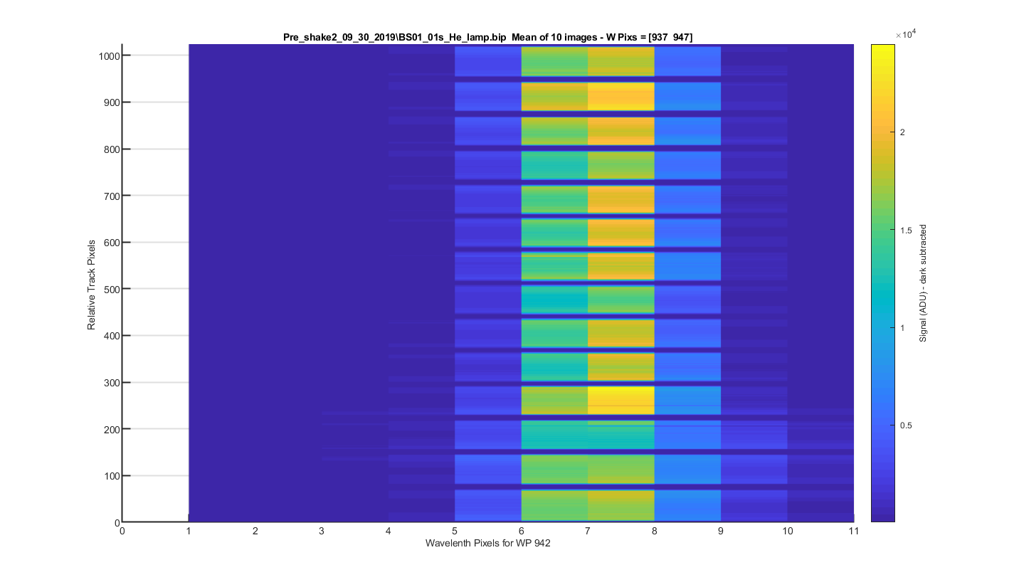
Figure 11 Helium Peak 5 (at pix 942): The same surface plot but showing how individual helium peaks line up from track to track.
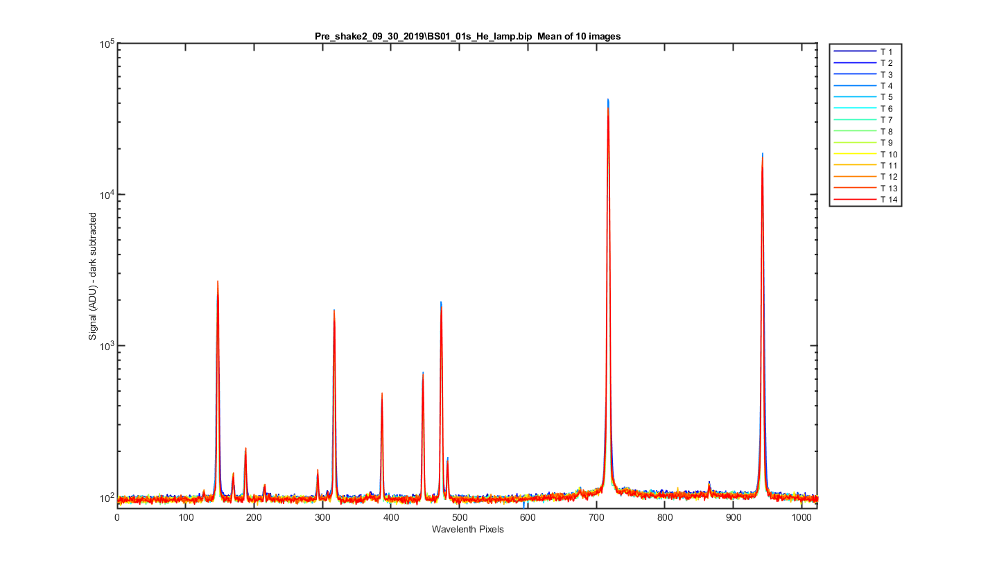
Figure 12 Mean image binned by track, the x-axis is wavelength pixels.
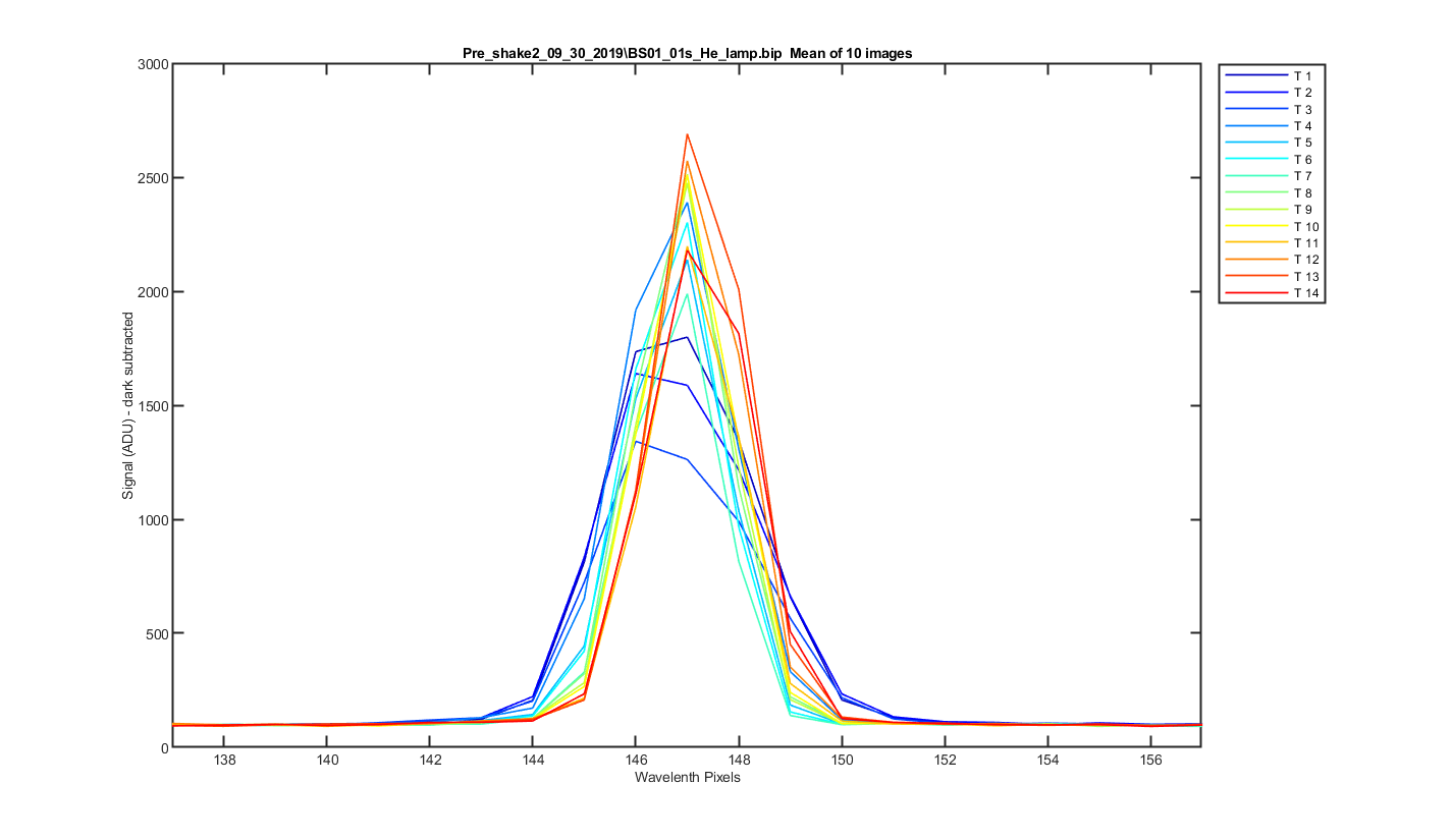
Figure 13 Close up of one of the helium peaks
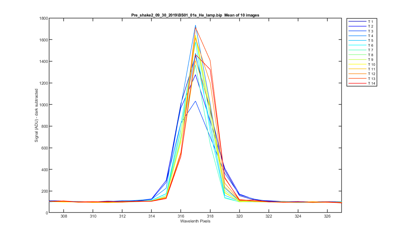
Figure 14 Close up of one of the helium peaks
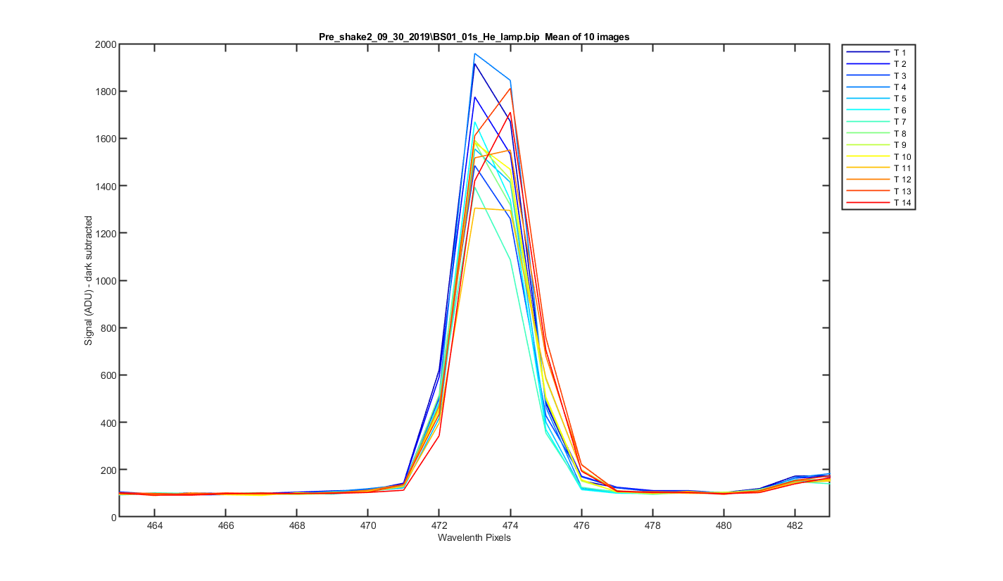
Figure 15 Close up of one of the helium peaks
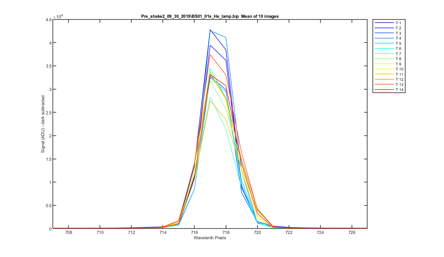
Figure 16 Close up of one of the helium peaks
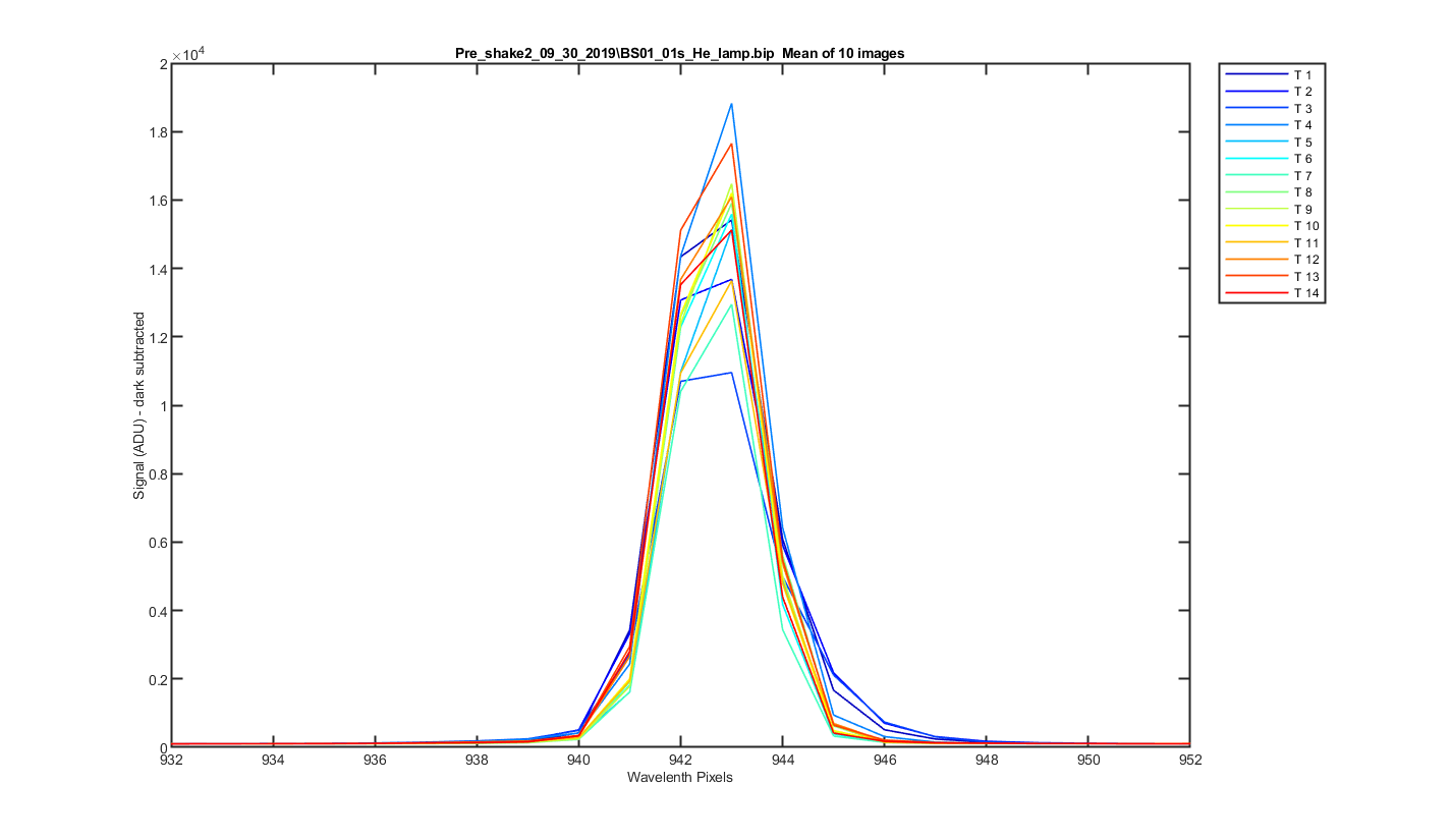
Figure 17 Close up of one of the helium peaks
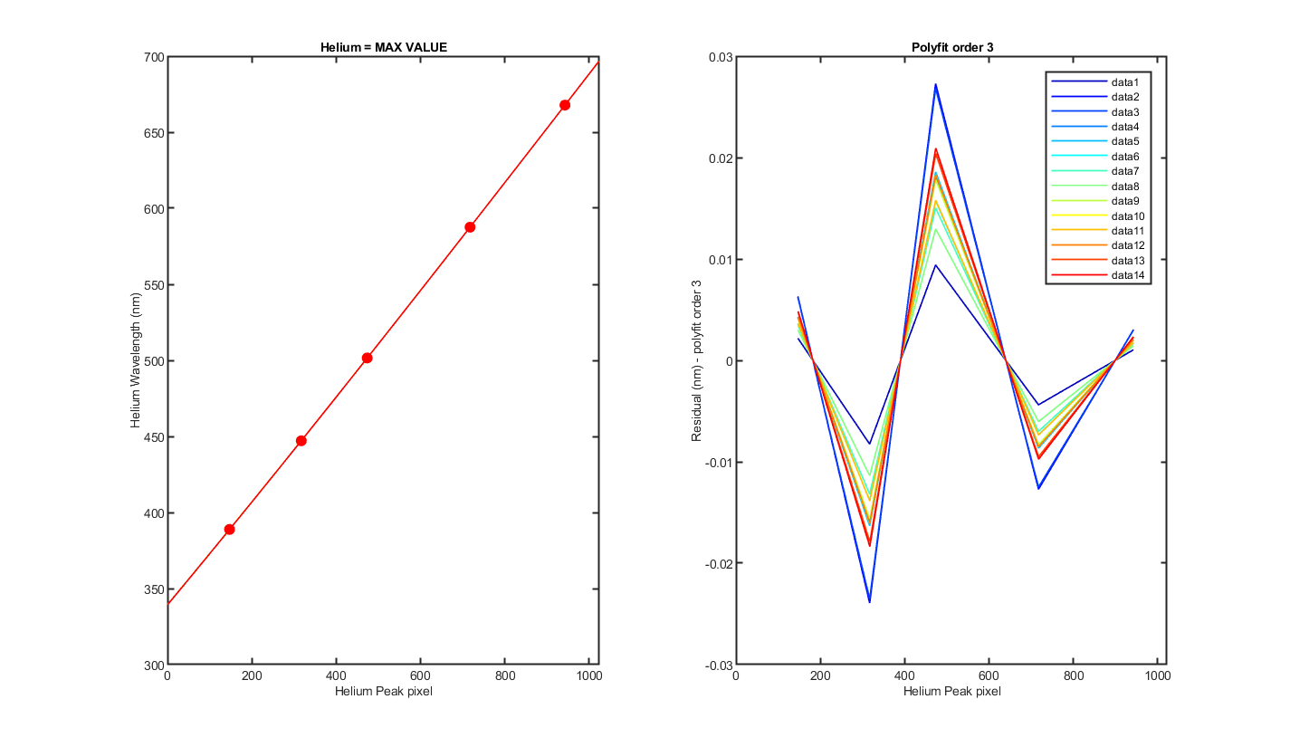
Figure 18 MY VERY ROUGH GUESS AT A WAVELENGTH CAL!!! THIS ASSUMES I GUESS CORRECTLY WHICH PEAKS WHERE WHICH HELIUM LINES.
Track, Min,    Max,     diff
    1, 339.74, 696.90,  0.35
    2, 339.81, 696.88,  0.35
    3, 339.82, 696.89,  0.35
    4, 339.79, 696.90,  0.35
    5, 339.78, 696.89,  0.35
    6, 339.78, 696.91,  0.35
    7, 339.78, 696.90,  0.35
    8, 339.74, 696.91,  0.35
    9, 339.72, 696.89,  0.35
   10, 339.70, 696.90,  0.35
   11, 339.65, 696.91,  0.35
   12, 339.63, 696.92,  0.35
   13, 339.60, 696.93,  0.35
   14, 339.61, 696.96,  0.35
  Track = The Resonon Track number
Lwave = Laser Wavelength
Lpix1 = Laser Pixel found using the max value of the track
Lpix2 = Laser Pixel found using mygaussfit to fit the laser peak
| Track | Lwave | Lpix1 | Lpix2 |
|---|---|---|---|
| 1 | 388.8648 | 147 | 146.86 |
| 1 | 447.148 | 317 | 316.98 |
| 1 | 501.5678 | 473 | 473.42 |
| 1 | 587.56 | 717 | 717.40 |
| 1 | 667.81 | 943 | 942.65 |
| 2 | 388.8648 | 146 | 146.81 |
| 2 | 447.148 | 317 | 317.08 |
| 2 | 501.5678 | 473 | 473.43 |
| 2 | 587.56 | 717 | 717.44 |
| 2 | 667.81 | 943 | 942.66 |
| 3 | 388.8648 | 146 | 146.78 |
| 3 | 447.148 | 317 | 317.06 |
| 3 | 501.5678 | 473 | 473.44 |
| 3 | 587.56 | 717 | 717.47 |
| 3 | 667.81 | 943 | 942.67 |
| 4 | 388.8648 | 147 | 146.77 |
| 4 | 447.148 | 317 | 317.01 |
| 4 | 501.5678 | 473 | 473.47 |
| 4 | 587.56 | 717 | 717.53 |
| 4 | 667.81 | 943 | 942.70 |
| 5 | 388.8648 | 147 | 146.79 |
| 5 | 447.148 | 317 | 317.02 |
| 5 | 501.5678 | 473 | 473.48 |
| 5 | 587.56 | 717 | 717.54 |
| 5 | 667.81 | 943 | 942.72 |
| 6 | 388.8648 | 147 | 146.77 |
| 6 | 447.148 | 317 | 316.97 |
| 6 | 501.5678 | 473 | 473.42 |
| 6 | 587.56 | 717 | 717.45 |
| 6 | 667.81 | 943 | 942.65 |
| 7 | 388.8648 | 147 | 146.79 |
| 7 | 447.148 | 317 | 316.97 |
| 7 | 501.5678 | 473 | 473.40 |
| 7 | 587.56 | 717 | 717.40 |
| 7 | 667.81 | 943 | 942.64 |
| 8 | 388.8648 | 147 | 146.88 |
| 8 | 447.148 | 317 | 317.05 |
| 8 | 501.5678 | 473 | 473.52 |
| 8 | 587.56 | 717 | 717.52 |
| 8 | 667.81 | 943 | 942.68 |
| 9 | 388.8648 | 147 | 146.94 |
| 9 | 447.148 | 317 | 317.11 |
| 9 | 501.5678 | 473 | 473.51 |
| 9 | 587.56 | 717 | 717.50 |
| 9 | 667.81 | 943 | 942.69 |
| 10 | 388.8648 | 147 | 146.99 |
| 10 | 447.148 | 317 | 317.14 |
| 10 | 501.5678 | 473 | 473.52 |
| 10 | 587.56 | 717 | 717.49 |
| 10 | 667.81 | 943 | 942.67 |
| 11 | 388.8648 | 147 | 147.11 |
| 11 | 447.148 | 317 | 317.23 |
| 11 | 501.5678 | 473 | 473.62 |
| 11 | 587.56 | 717 | 717.55 |
| 11 | 667.81 | 943 | 942.67 |
| 12 | 388.8648 | 147 | 147.17 |
| 12 | 447.148 | 317 | 317.28 |
| 12 | 501.5678 | 474 | 473.61 |
| 12 | 587.56 | 717 | 717.50 |
| 12 | 667.81 | 943 | 942.63 |
| 13 | 388.8648 | 147 | 147.25 |
| 13 | 447.148 | 317 | 317.35 |
| 13 | 501.5678 | 474 | 473.66 |
| 13 | 587.56 | 717 | 717.54 |
| 13 | 667.81 | 943 | 942.62 |
| 14 | 388.8648 | 147 | 147.24 |
| 14 | 447.148 | 317 | 317.38 |
| 14 | 501.5678 | 474 | 473.70 |
| 14 | 587.56 | 717 | 717.57 |
| 14 | 667.81 | 943 | 942.58 |