REVISION DATE: 29-Apr-2016 16:55:03
The Heilum wave cal data. The darks where at lest 650 ADU to high so subtracted 650 ADU from the darks. This is not quite right but works.
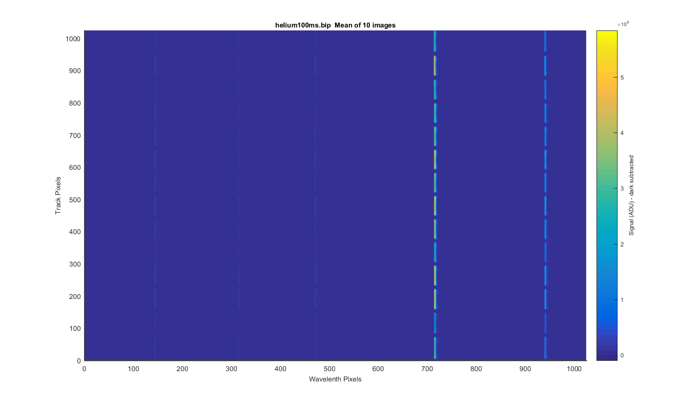
Below are my graphs of the helium 100ms data. The file contains 10 images of the helium lamp source. All the data are dark subtracted. See each graph below for more detail.
Track Wavelength fits:
P(1,:) = [1.302214e-05     0.3369538      339.8327]
P(2,:) = [1.21057e-05     0.3377253      339.7133]
P(3,:) = [1.153468e-05     0.3381601      339.7595]
P(4,:) = [1.055377e-05     0.3393074      339.5041]
P(5,:) = [1.153592e-05     0.3384246      339.4908]
P(6,:) = [1.210172e-05     0.3375175      339.8749]
P(7,:) = [1.17737e-05     0.3377634      339.9243]
P(8,:) = [1.144687e-05     0.3381925      339.7818]
P(9,:) = [1.146954e-05     0.3382023      339.7311]
P(10,:) = [1.13485e-05     0.3383441      339.6533]
P(11,:) = [1.134945e-05      0.338363      339.6437]
P(12,:) = [1.168079e-05     0.3381153      339.7227]
P(13,:) = [1.132644e-05     0.3385015      339.7169]
P(14,:) = [1.139838e-05     0.3384457      339.7307]
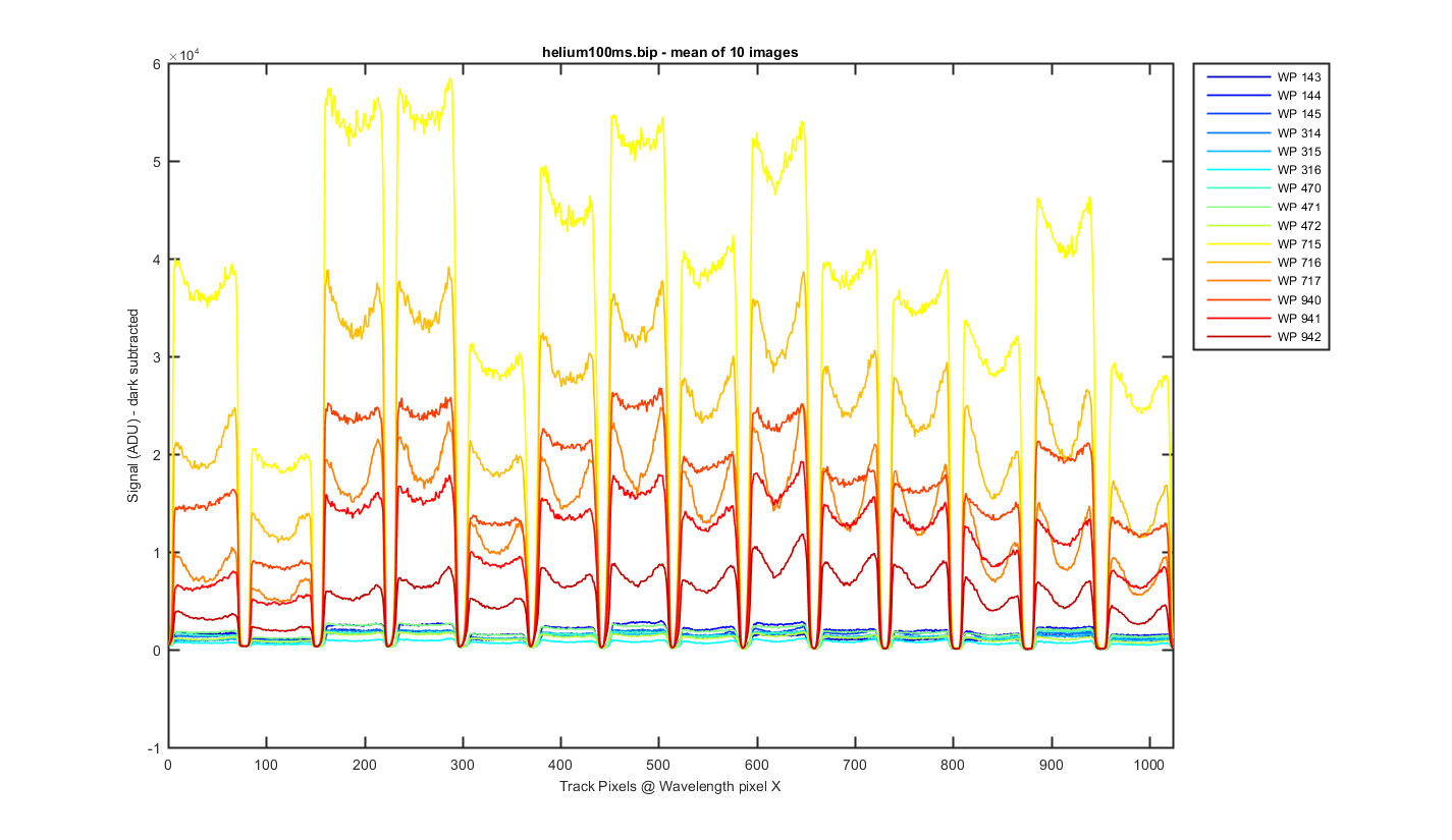
Resonon took dark scans for the two int times taken. So I meaned all the dark images for the 100ms data and subtracted it from the data before processing. I Then took the 10 images and meaned them to get the surface plot below.
Figure 1
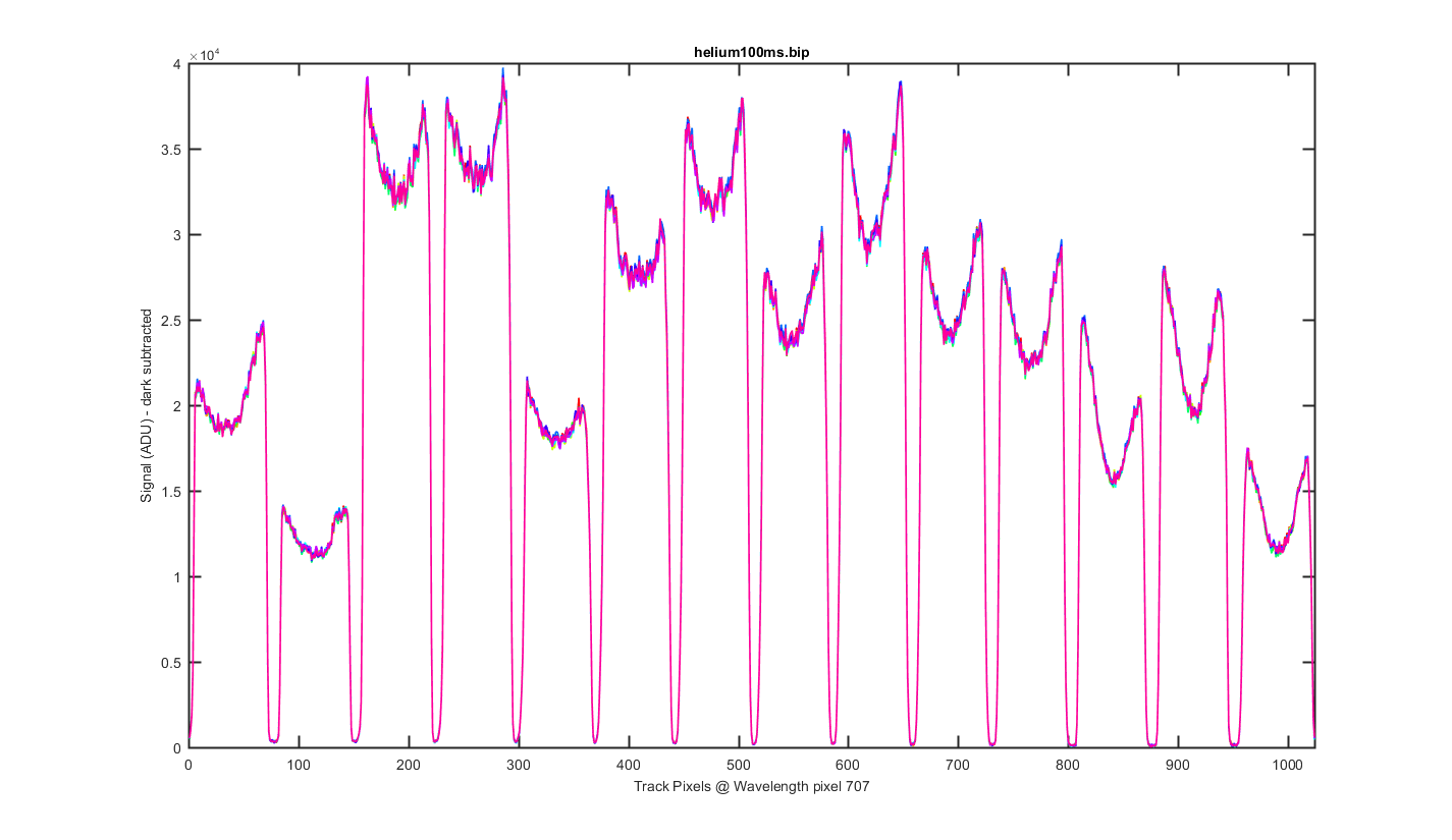
This is a cross section through the tracks at wavelength pixel 716, with one line for each of the 10 images. The tracks and their shapes look really stable.
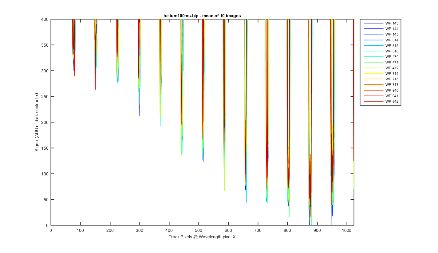
Figure 2
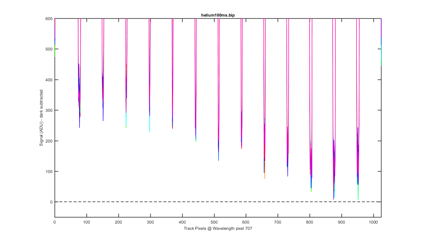
Same as the previous graph but zoomed into the bottom to see the level of the darks between the tracks. I had to subtract 650 ADU from the darks to make them work.
Figure 3
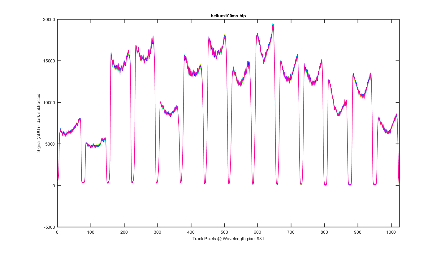
Same as figure 2 but for Wavelength pixel 941.
Figure 4
Again this is the mean image with slices thought the image at different wavelength pixels. The pixels choosen are where the helium peaks are and +- pixel pixel around them.
Figure 5
Same as figure 5 but zoomed to the bottom so you can see the darks between the tracks.
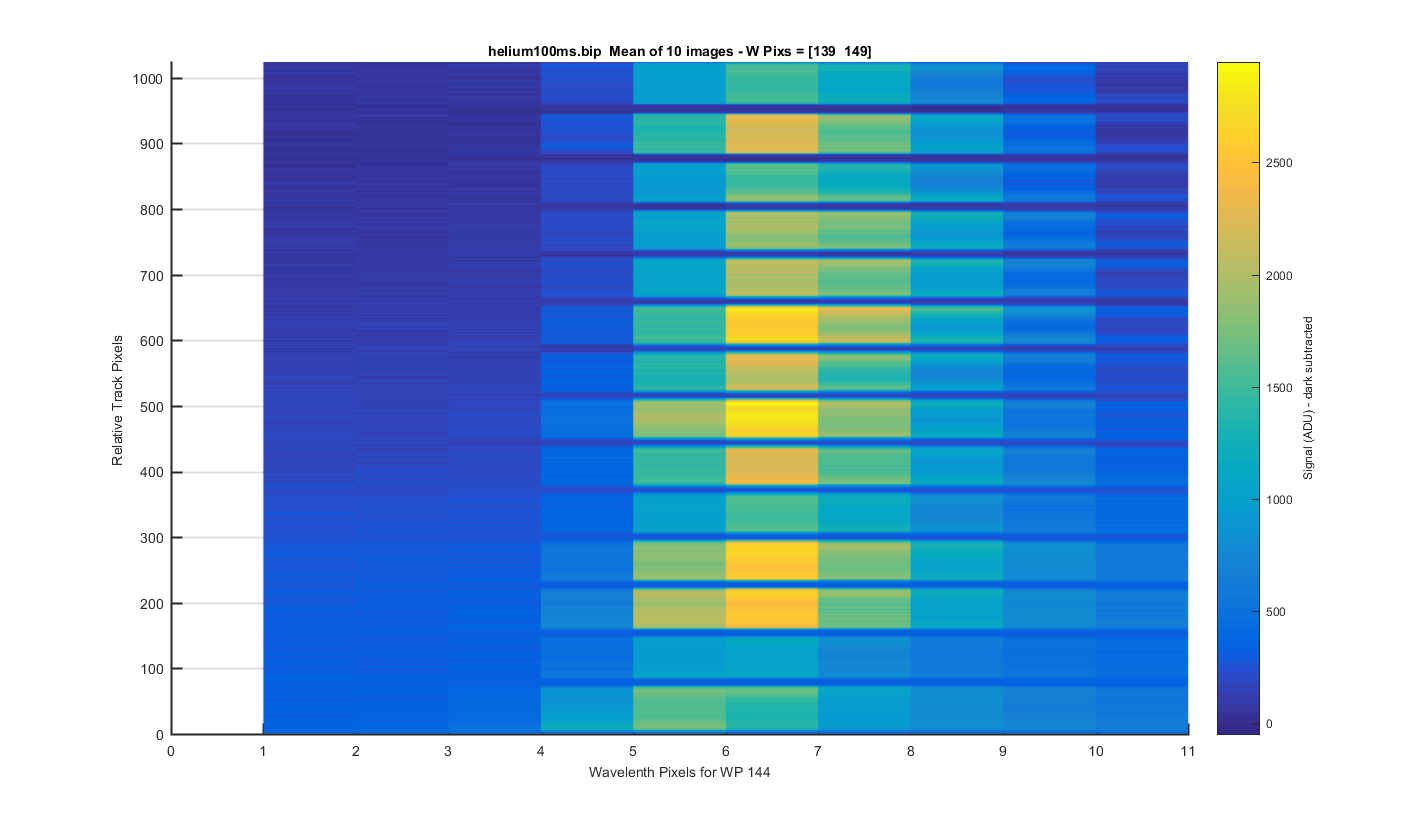
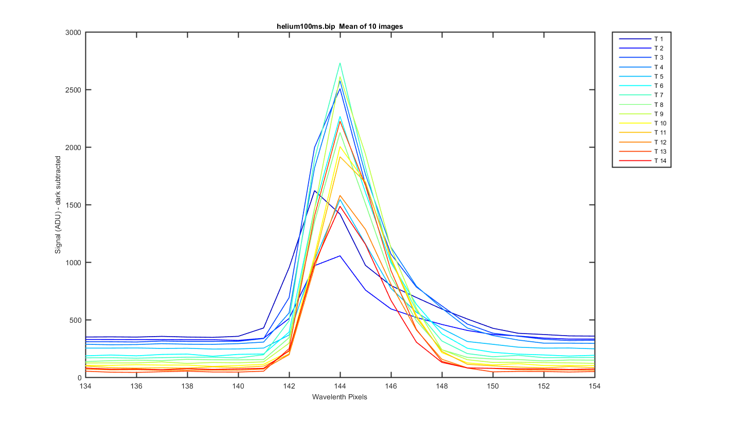
Figure 6
Helium Peak 1 (at pix 144): The same surface plot but showing how individual helium peaks line up from track to track.
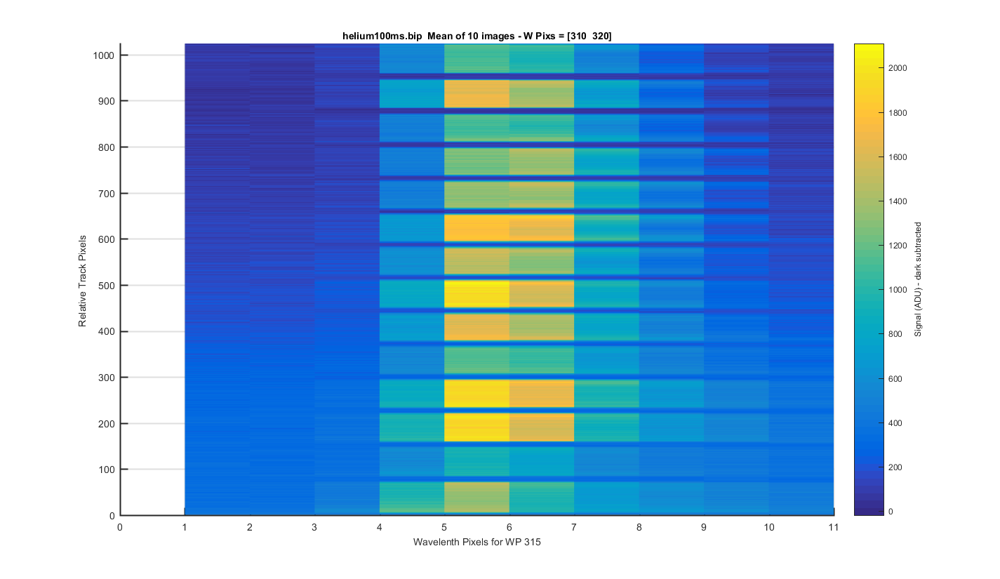
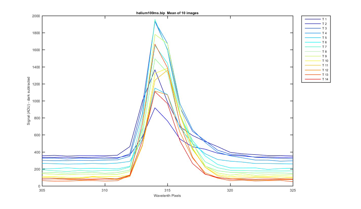
Figure 7
Helium Peak 2 (at pix 315): The same surface plot but showing how individual helium peaks line up from track to track.
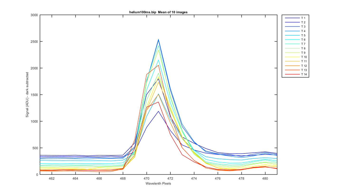
Figure 8
Helium Peak 3 (at pix 471): The same surface plot but showing how individual helium peaks line up from track to track.
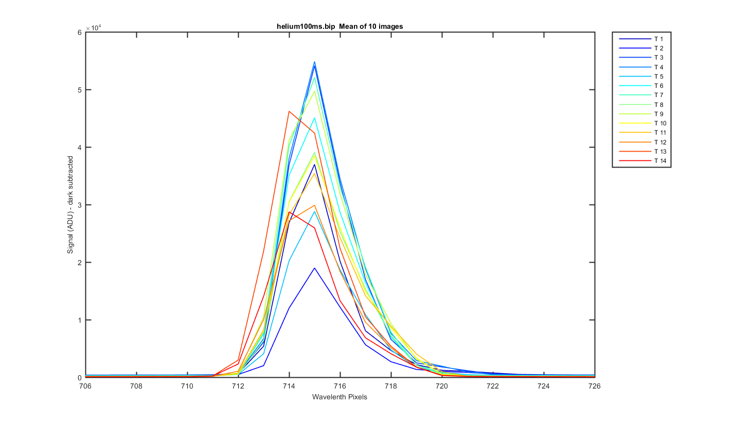
Figure 9
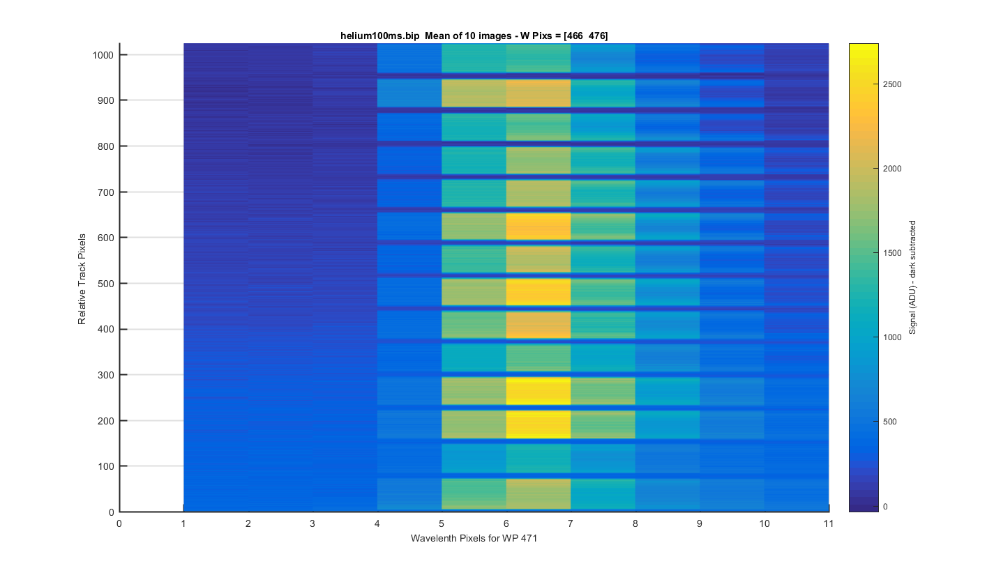
Helium Peak 4 (at pix 716): The same surface plot but showing how individual helium peaks line up from track to track.
Figure 10
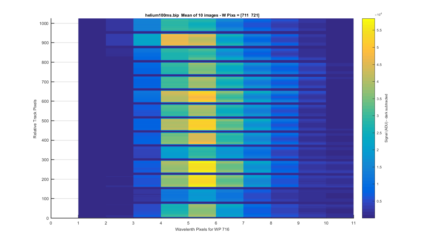
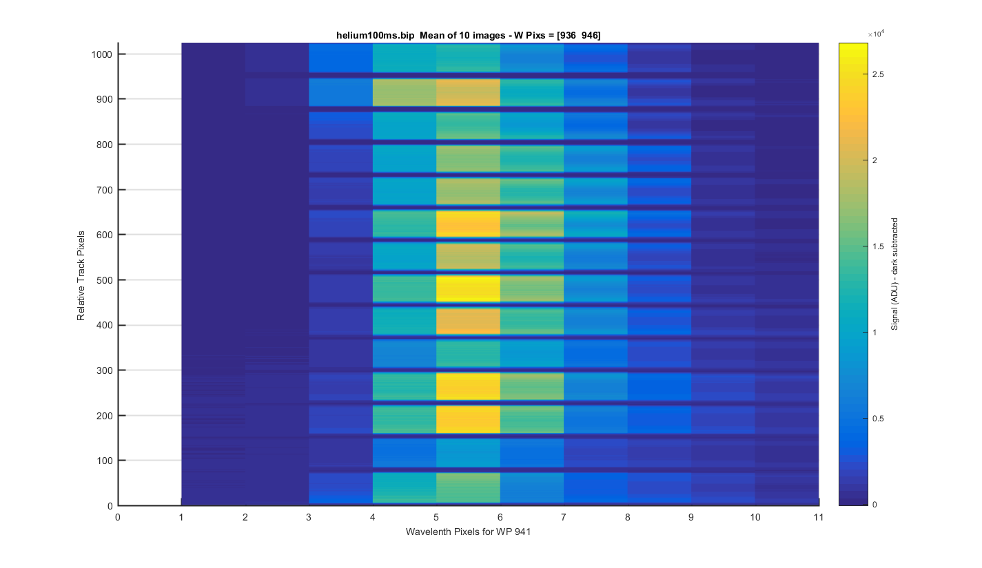
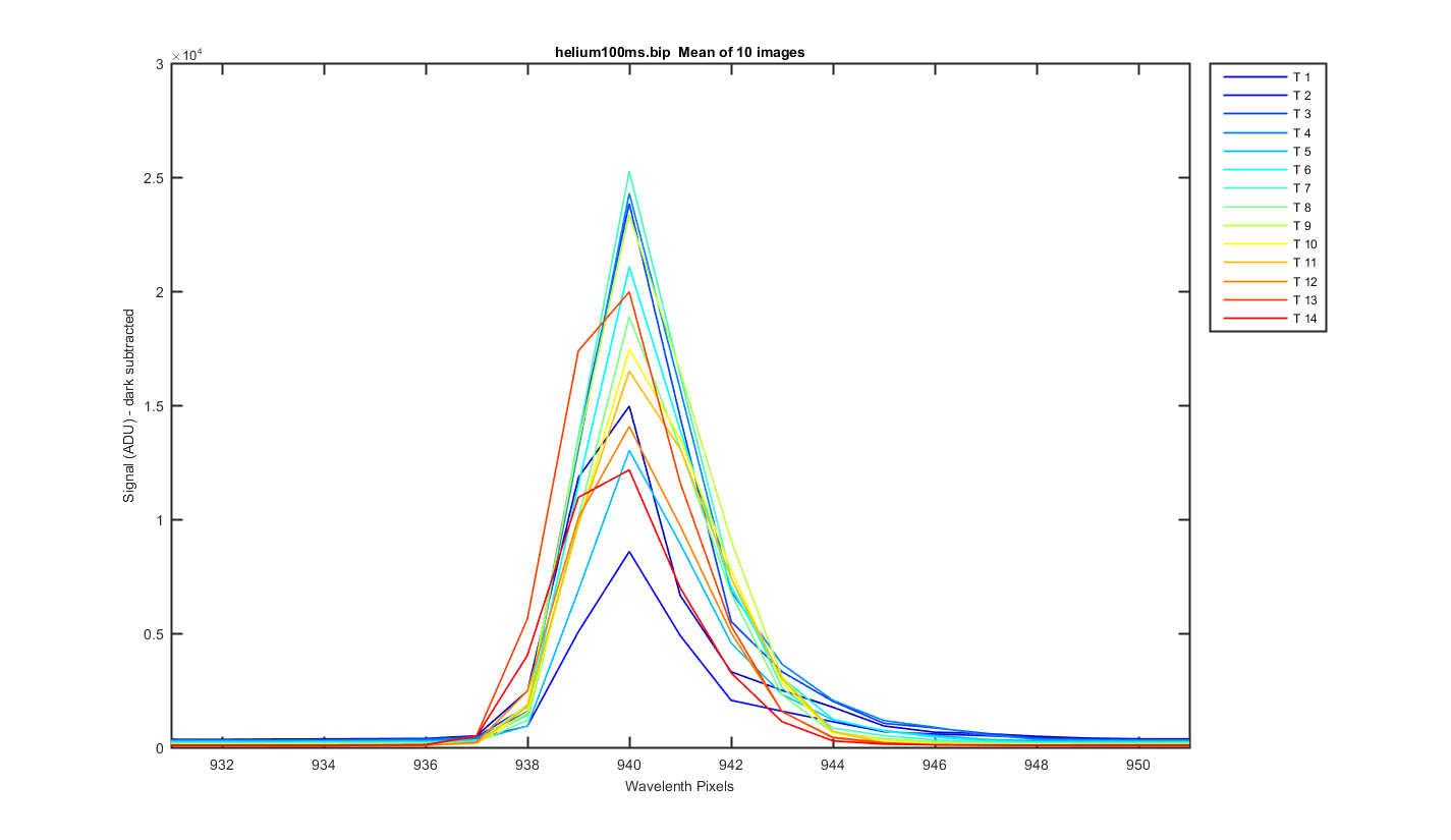
Helium Peak 5 (at pix 941): The same surface plot but showing how individual helium peaks line up from track to track.
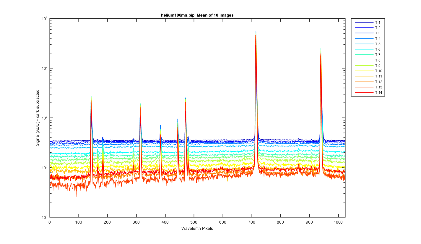
Figure 11
Mean image binned by track, the x-axis is wavelength pixels. The darks going up in the back are because subtracking 650 ADU is not quite the right way to correct the darks.
Figure 12
Close up of one of the helium peaks
Figure 13
Close up of one of the helium peaks
Figure 14
Close up of one of the helium peaks
Figure 15
Close up of one of the helium peaks
Figure 16
Close up of one of the helium peaks
Figure 17
MY VERY ROUGH GUESS AT A WAVELENGTH CAL!!! THIS ASSUMES I GUESS CORRECTLY WHICH PEAKS WHERE WHICH HELIUM LINES.
Track, Min,    Max,     diff
    1, 340.17, 698.53,  0.35
    2, 340.05, 698.24,  0.35
    3, 340.10, 698.13,  0.35
    4, 339.84, 698.02,  0.35
    5, 339.83, 698.13,  0.35
    6, 340.21, 698.18,  0.35
    7, 340.26, 698.14,  0.35
    8, 340.12, 698.09,  0.35
    9, 340.07, 698.08,  0.35
   10, 339.99, 698.02,  0.35
   11, 339.98, 698.03,  0.35
   12, 340.06, 698.20,  0.35
   13, 340.06, 698.22,  0.35
   14, 340.07, 698.25,  0.35
Figure 18
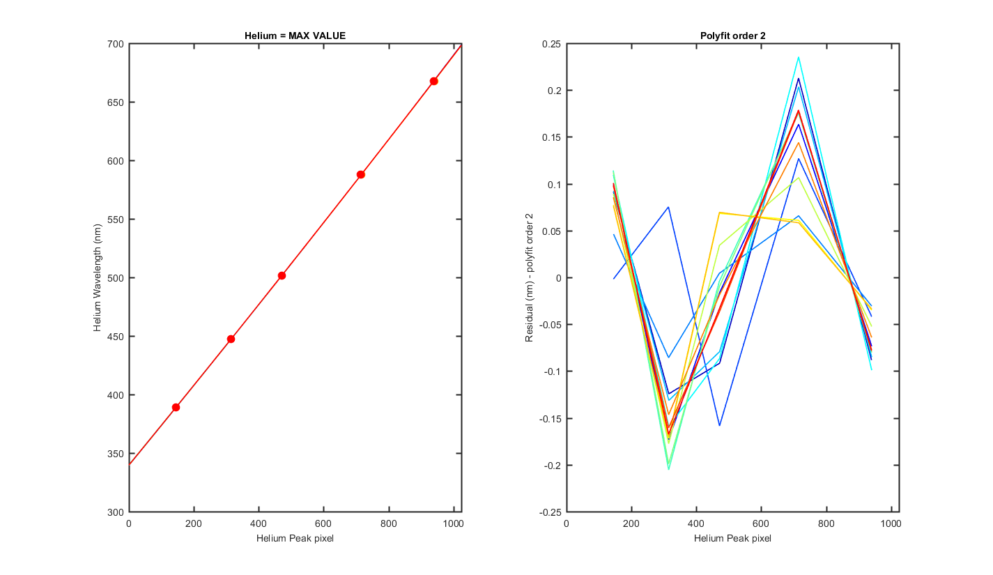
  Track = The Resonon Track number
Lwave = Laser Wavelength
Lpix1 = Laser Pixel found using the max value of the track
Lpix2 = Laser Pixel found using mygaussfit to fit the laser peak
| Track | Lwave | Lpix1 | Lpix2 |
|---|---|---|---|
| 1 | 388.8648 | 143 | 144.44 |
| 1 | 447.148 | 314 | 315.02 |
| 1 | 501.5678 | 471 | 471.67 |
| 1 | 587.56 | 715 | 714.82 |
| 1 | 667.81 | 940 | 939.51 |
| 2 | 388.8648 | 144 | 144.49 |
| 2 | 447.148 | 314 | 315.07 |
| 2 | 501.5678 | 471 | 471.33 |
| 2 | 587.56 | 715 | 715.06 |
| 2 | 667.81 | 940 | 940.03 |
| 3 | 388.8648 | 144 | 144.51 |
| 3 | 447.148 | 314 | 313.98 |
| 3 | 501.5678 | 471 | 471.39 |
| 3 | 587.56 | 715 | 714.98 |
| 3 | 667.81 | 940 | 940.08 |
| 4 | 388.8648 | 144 | 144.69 |
| 4 | 447.148 | 314 | 314.42 |
| 4 | 501.5678 | 471 | 470.73 |
| 4 | 587.56 | 715 | 714.97 |
| 4 | 667.81 | 940 | 940.17 |
| 5 | 388.8648 | 144 | 144.91 |
| 5 | 447.148 | 314 | 315.12 |
| 5 | 501.5678 | 471 | 471.57 |
| 5 | 587.56 | 715 | 714.99 |
| 5 | 667.81 | 940 | 940.26 |
| 6 | 388.8648 | 144 | 144.08 |
| 6 | 447.148 | 314 | 314.75 |
| 6 | 501.5678 | 471 | 471.36 |
| 6 | 587.56 | 715 | 714.82 |
| 6 | 667.81 | 940 | 940.21 |
| 7 | 388.8648 | 144 | 143.84 |
| 7 | 447.148 | 314 | 314.61 |
| 7 | 501.5678 | 471 | 470.85 |
| 7 | 587.56 | 715 | 714.83 |
| 7 | 667.81 | 940 | 940.18 |
| 8 | 388.8648 | 144 | 144.10 |
| 8 | 447.148 | 314 | 314.71 |
| 8 | 501.5678 | 471 | 470.91 |
| 8 | 587.56 | 715 | 714.84 |
| 8 | 667.81 | 940 | 940.26 |
| 9 | 388.8648 | 144 | 144.31 |
| 9 | 447.148 | 314 | 314.78 |
| 9 | 501.5678 | 471 | 470.90 |
| 9 | 587.56 | 715 | 715.12 |
| 9 | 667.81 | 940 | 940.24 |
| 10 | 388.8648 | 144 | 144.52 |
| 10 | 447.148 | 315 | 314.89 |
| 10 | 501.5678 | 471 | 470.91 |
| 10 | 587.56 | 715 | 715.36 |
| 10 | 667.81 | 940 | 940.34 |
| 11 | 388.8648 | 144 | 144.54 |
| 11 | 447.148 | 315 | 314.90 |
| 11 | 501.5678 | 471 | 470.91 |
| 11 | 587.56 | 715 | 715.36 |
| 11 | 667.81 | 940 | 940.31 |
| 12 | 388.8648 | 144 | 144.37 |
| 12 | 447.148 | 314 | 314.73 |
| 12 | 501.5678 | 471 | 471.06 |
| 12 | 587.56 | 715 | 714.91 |
| 12 | 667.81 | 940 | 940.01 |
| 13 | 388.8648 | 144 | 144.21 |
| 13 | 447.148 | 314 | 314.54 |
| 13 | 501.5678 | 471 | 470.83 |
| 13 | 587.56 | 714 | 714.57 |
| 13 | 667.81 | 940 | 939.92 |
| 14 | 388.8648 | 144 | 144.18 |
| 14 | 447.148 | 314 | 314.55 |
| 14 | 501.5678 | 471 | 470.81 |
| 14 | 587.56 | 714 | 714.53 |
| 14 | 667.81 | 940 | 939.85 |