While in Oregon at the AGU conference, Al Parr and I were discussing the MOBY straylight and some of the issues in the UV area. While discussing this with Al we were trying to balance the issue of low signal (so high uncertainties) with the getting the correction as correct as possible. For the Even buoy for the few files I have run the new correction and the change to the 412 nm band is around 6.5%. This is on top of the original straylight correction! That is big, we need to do some checking! 6.5% seems too high but when you look at the spectral data the UV gets even higher, for the odd buoy the change to 412 nm is 4.9%. Were do you start looking to see if this is correct or not?? Al had a brilliant thought about how to think of the problem. Think of each row of the SPR like a satellite band then look where the biggest "out-of-band" areas are. So this webpage is my attempt to look at that issues and figure out were I need to spiff the SPR to get a better handle on the SPRs effect on the UV.

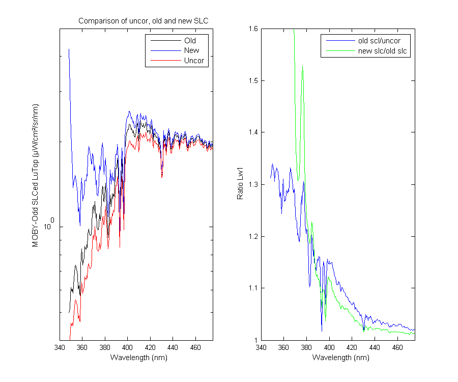
The graph below shows some MOBY data straylight corrected with the old and new SLC and uncorrected. You can see that the new SLC raises the UV significantly. This of course affects the satellite 412 nm band ALOT! So the first question is is this right? Is the UV really that high and we have been getting it wrong all this time? Or is the new SLC too high in the UV. I plotted some of MikeO's SLC hyperpro data from the M234 cruise. When plotting absolute values there was a lot of variablity but if you just compared the spectral shape of MOBY and the hyperpro data is looked really good. The only part which stood out was the first few pixels on the UV end which are too high.

Figure 1

This is a zoomed view of the UV region so you can see the problem better. The complication of course is we don't have any old laser data in the UV region to compare to the new laser data. The high pixels on the UV end are the first 5-6 pixels.

Figure 2

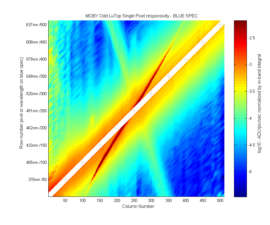
This is the single pixel responsivity or stray light correction matrix. Columns are the laser data, 60 are measured laser scans (smoothed) the rest are interpolated laser data. Each laser was normalized by it's own in-band area before interpolation. Laser data describes how that wavelength of light affects all the other pixels. Ie how much straylight that one wavelength contributes to the other wavelengths. What we need is the reverse; how all the other wavelengths affect this one wavelength. That is the rows in the image below.

I am not sure if this is totally correct but if you think of each row like a satellite band where the main peak (white area) is the "in-band" and the rest of the row as the "out-of-band" or stray light. If you think of the data this way then you can look for the "out-of-band" area which might contribute the most to the incorrect value in each pixel. This should tell use were to focus the my efforts in creating a SPR matrix.

Keep in mind, there are a lot of features to be interpolated, 2 reflection peaks and large bumps. The dark red streak is the reflection peak, the cyan/yellow strip which goes from column 350 to 200 almost perpendicular to the main peak (white area) is the large hump which transects the spectragraph. The double bump seen in the upper left in the even buoy is not really seen in the odd buoy. How well each of these need to me interpolated is one question. Since the "large" bump is smaller in the odd buoy then in the even buoy. Ahd because "fixing" the interpolation of the large bump in the even buoy had a very small effect I am ignoring the large bump.

Figure 3

In-water data: The following will show how the straylight correction affects the in-water data.

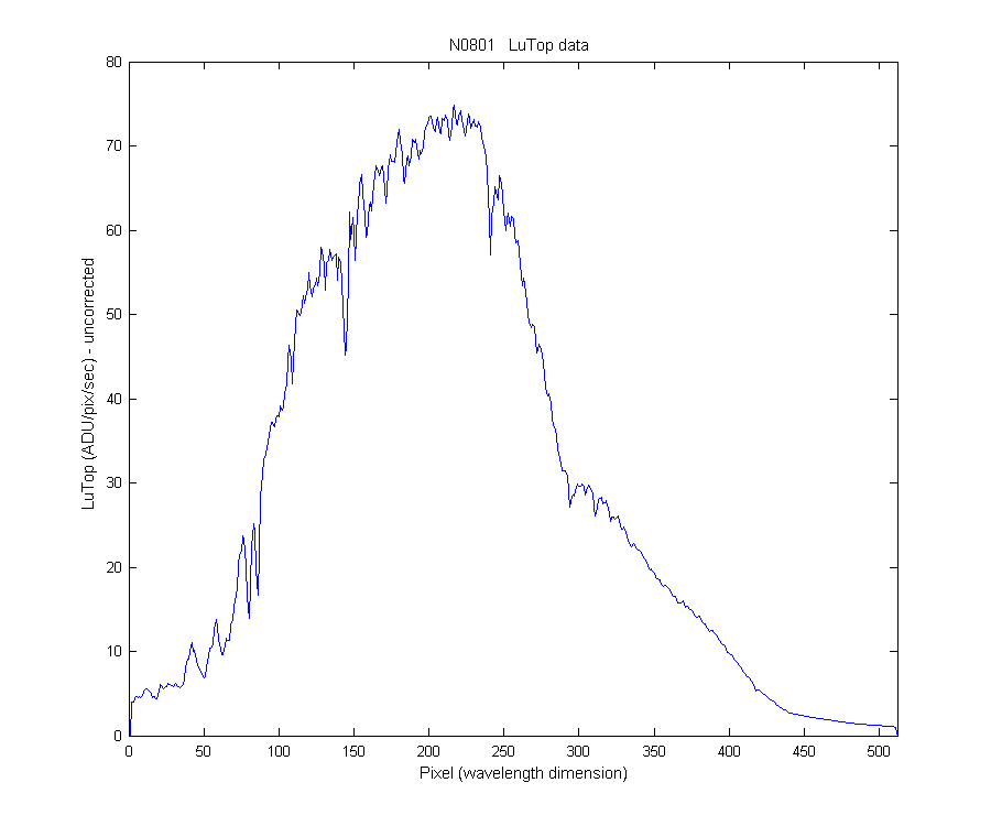
This graph is of the uncorrect LuTop signal (ADU/pixel/sec) or Lo in the equations to follow. With some matrix math magic the SPR above and the LuTop signal below is mashed together and out comes the straylight corrected LuTop signal. Notice the very low value at pixel 1.

Figure 4

The green line is the answer, the stray light corrected in-water data. This does not have the system response applied so the LuTop does down (no up as seen when the system response is applied) . I think I should make this clearer. When the SLC is applied to any data (ADU/pix/sec) the answer is always less than the uncorrected signal. This applies to in-water and lamp calibration signal. You then use the SLC lamp signal to create a system response and then apply it to the in-water SLCed signal. Because the spectral difference in the sources (in-water blue rich, cal lamp red rich) the converted Lu in-water data can go up or down. Ie the UV is higher for the straylight correct in-water data.

Figure 5

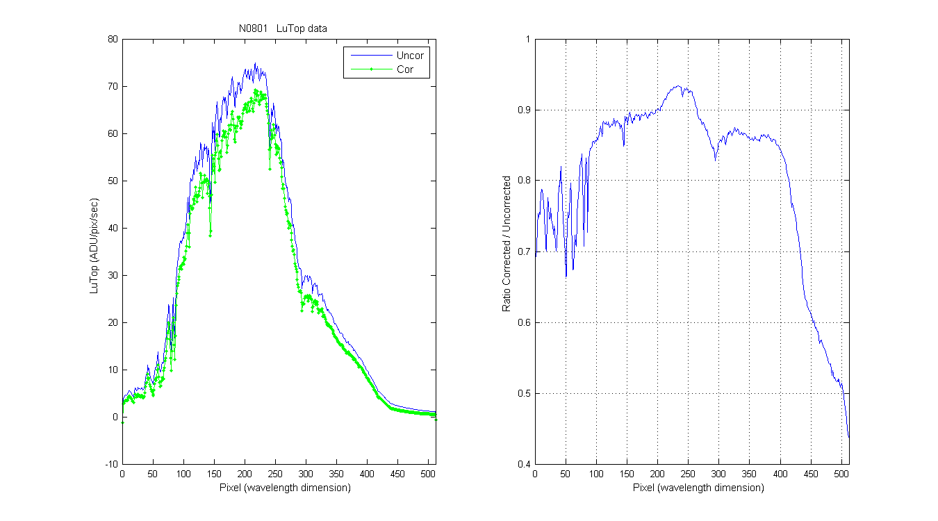
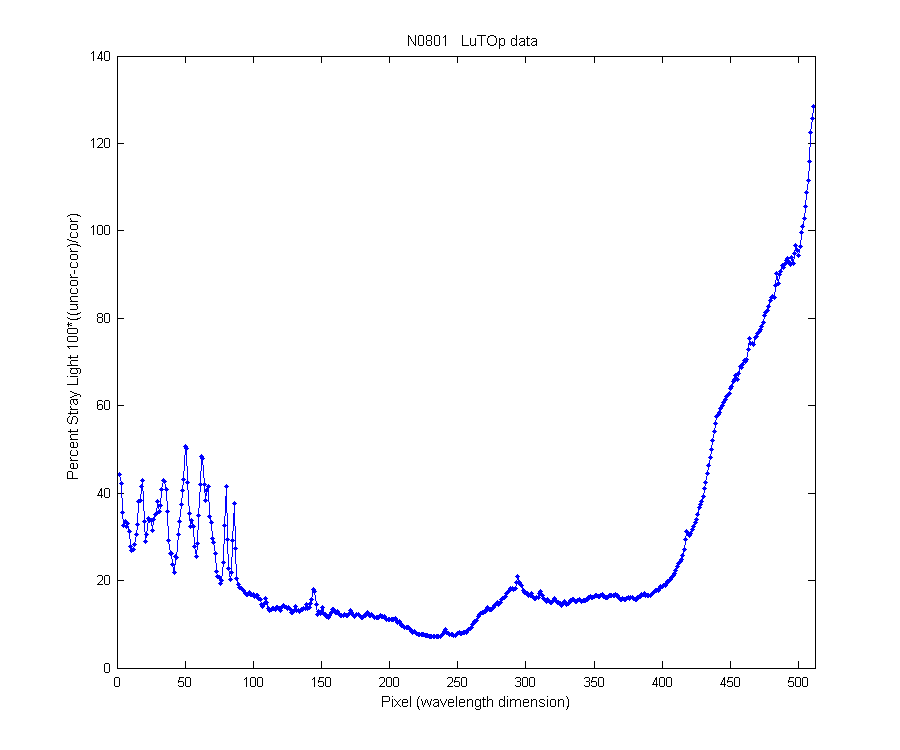
This shows spectrally the percent of the signal which is stray light.

Figure 6

I have always understood this process from a conceptual point of view but now I need to understand the nitty gritty math so I can do the matrix math manually.

The process begins with me pulling out my Precalculus book to look up matrix math (painful and oh so long ago). Below are some equations I started with.

Matlab help on use of inv function: In practice, it is seldom necessary to form the explicit inverse of a matrix. A frequent misuse of inv arises when solving the system of linear equations . One way to solve this is with x = inv(A)*b. A better way, from both an execution time and numerical accuracy standpoint, is to use the matrix division operator x = A\b. This produces the solution using Gaussian elimination, without forming the inverse. See \ and / for further information.

The problem is that at this point what you get is the spectral straylight corrected answer but what I want is the matrix before it is summed. I used a for loop to create the weighted matrix.

A = inv((eye(512,512) + SPR)); % add ones on diagional and invert
for k = 1:512
  SPRw(:,k) = A(:,k)*Lo(k,1);
end

At the bottom of this page is the image of the matrix A.

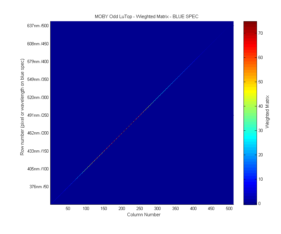
The image below shows the weighted matrix (ADU/pix/sec) , you can see that most of the signal is in the diagonal in-band area. If you sum each row you get the stray light corrected answer. Note: The bright dots down the diagonal are not real and don't exist in the Matlab figure intil printed.

Just to make sure we are clear. This image is created by taking column 1 in figure 3 and multiplying it by pixel 1 in Figure 4, and then repeating this for each column in Figure 3 and pixel in Figure 4. Resulting in Figure 7. Note also that each Row in Figure 7 coresponse to one pixel on the blue spectrograph. Also note that the units are (ADU/pix/sec) because the sum is the corrected answer in (ADU/pix/sec).

Figure 7

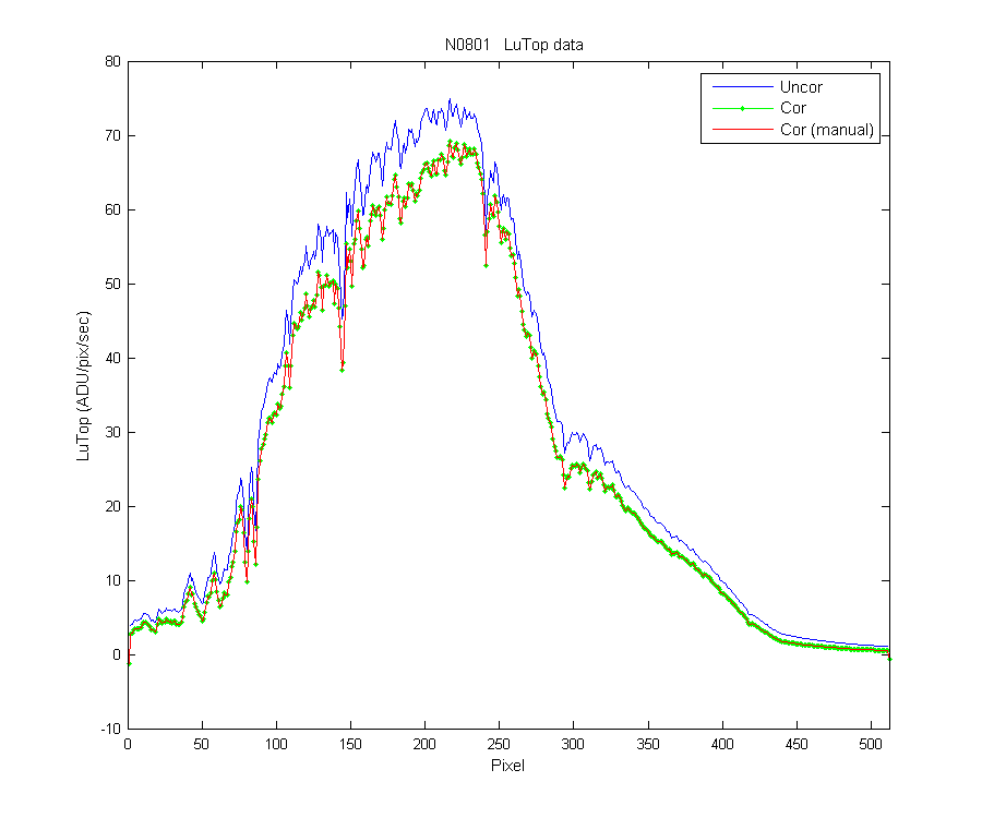
To check to make sure I had done the math right I summed each row and plotted the manual corrected data below. Looks good.

Figure 8

Next I wanted to look at the out-of-band data and replot the weighted matrix in some meaningful way. Here is were I got really stuck, I could not figure out how to get what I wanted. So I called Mike F. and he helped be get a handle on what this means and how to plot it. Thanks Mike.

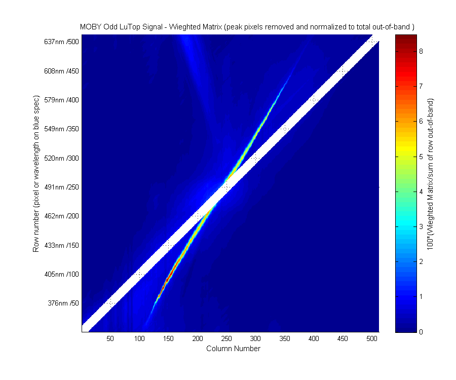
So I removed the in-band data, and divided each row by the sum of that row and multiplied by 100. The sum of that row (with the in-band removed) is the total straylight. So what I ended up with is a image of the percent of the total straylight for each pixel row by row. The image below shows the percent straylight of the wieghted matrix.

Figure 9

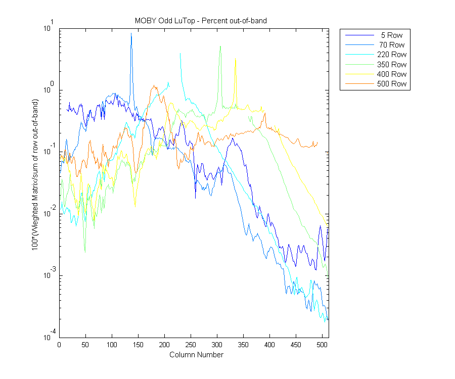
To look at this row by row Mike and I picked a few rows with interesting features in them. The below plot is the line plot of the image above. Now it is a little easier to see which area of the spectrum contributes the most to the straylight for any row in the matrix, which is a one pixel/wavelength in the straylight corrected spectrum.

Figure 10

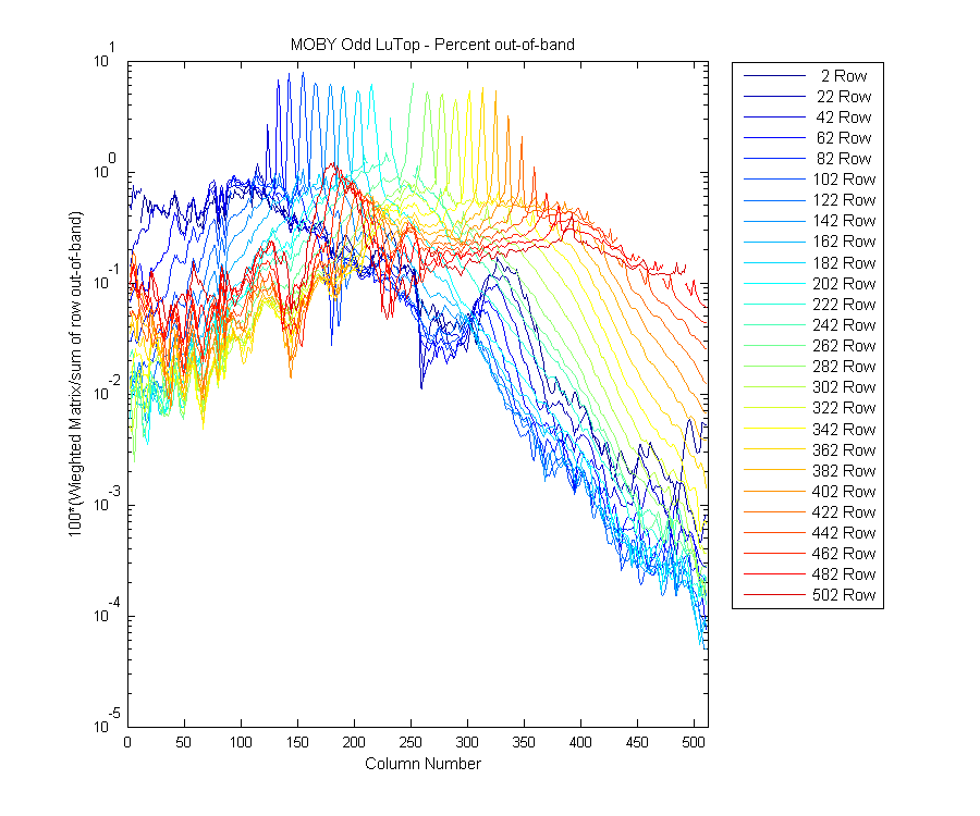
Same graph as above but for more wavelengths.

Figure 11

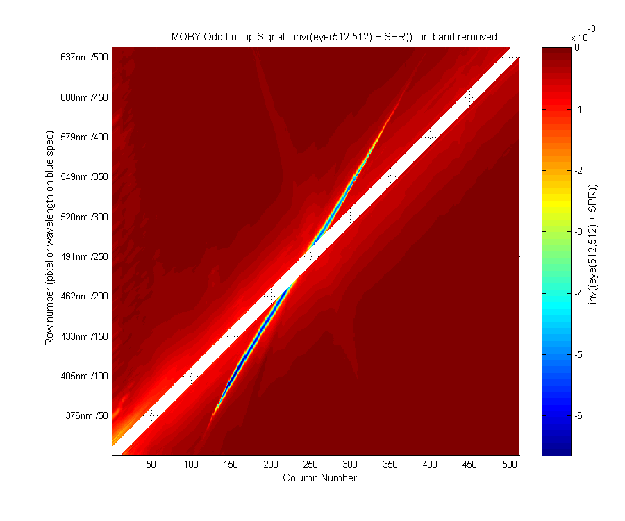
This is the Matrix A (A = inv((eye(512,512) + SPR))) with the in-band area removed.

Figure 14