plt_linearity3_
REVISION DATE: 26-Feb-2013 15:14:29
Who would have thought linearity was so hard, ARGH. Using Carol's linearity write up
and after talking to Carol to make sure I understood I started setting up the matrices to do solve the linear equations.
Also reading the Saunders and Shumaker (1984) paper
is helpful. I will decribe below the way I set up the matrices and my understanding of how it works. You should be able
to follow along using Carol write-up.
One thing to note is that I removed the OH,H aperatures so there are 27 not 29 rows in s and U. This means that
s 27 by 1 and U is 27 by 16 (not 17). Removing the two aperatures got rid of the single aperature H and therefore one of the φ.
The φ's are unknowns. φ is the contribution of the total flux from the a aperature. THere is a φ for each of the single aperatures, no doubles.
For example for aperature readings A,IA,I,IB,B,JB,J only A, I, B and J have an unknown φ
r is the other unknown and is coefficents of the response function.
EQUATIONS 1:
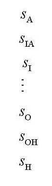
S are the net values near the max for each aperature (all 27 measurements).
They were called RD in the other linearity pages and in the GS5000 manual worksheet.
The OH and H shown below are not used in the calcuations.
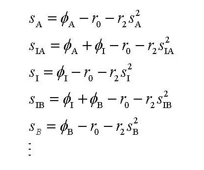
EQUATIONS 2:
Equations used to create the U matrix. The row coresponds to which S is being solved for and
the column is which φ is in the S's equation and the r coeff's.
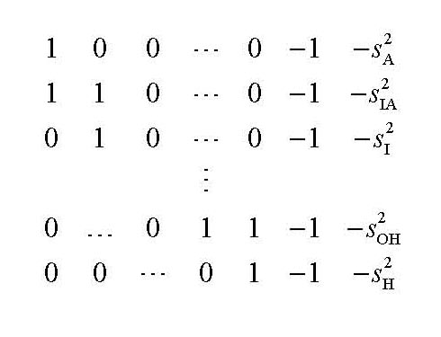
EQUATIONS 3:
Ok so here is the harder one to explain. Row 1 in U is for Sa and the first 14 columns are either 0 or 1
if φ is in the equations. col1 = φA, col2 = φI, col3 = φB and so on. So if
U(1,1) = 1 then φA is in the Sa equation. If U(2,1) and U(3,1) = 1 then φA and φI is in
the equation. U(:,15) are all -1 for the ro in the equations and U(:,16) are the Sx values squared.
EQUATIONS 4:
These are the unknowns we are solving for. This is the order the matrix math returns the φ and r's.
I should not that there are no φ's for φIA or φJB... because the φ's are only the single aperature data.
They are the unknowns we are trying to solve for.
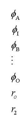
You then take the S and U variables and do some matrix math magic which returns the φ and r's in equations 4 above.
φ and r's = (inv(U'*U)*U')*S . These are shown in the table below.
To understand the data and how Mike collected it look at the GS5000 manual
Mike Linearity email 1
I ran Es with the GS5000-14 Linearity Assembly, "which allows the measurement of a detector's amplitude response (linearity) relative to incident
radiant flux". This Assy. has 15 different diameter apertures which are rotated into the beam of an FEL lamp. Apertures are selected either one at a time, or a pair together,
so that the detector sees a small aperture, a large aperture, or both together. When both are viewed, the measured signal
should equal the sum of the signals from the two individual apertures.
They are available for your Gbridge access:
GS5000-14_manual_2.pdf = manual
GS5000-14_linearity_*.jpg = photos of setup
FEL-GS922_*.jpg = photos of the (retired) FEL
Oahu13_ResCalLogMF_24 & 25.png = log sheet scans
R & R*.txt & .SPE = FISH data
I've only run this once before with MOS205 LuMOS via an integrating sphere, so it will be interesting to see how/if
this works with a cosine collector. The second-to-last page of the GS5000-14 manual shows a filled-in log-sheet that
gives an example how "linearity" can be determined.
Mike Linearity email 2
One more ting:
The way I ran this "experiment" was to scan all GS light levels at one FISH gain/exposure setting,
so that we see how (A+B) = A + B from low ADU through high ADU, independent of camera "gain".
I.E. check camera gain throughout the range of the 16 A/D: ~0 ADU to ~40k ADU.
PDF papers on linearity:
GS5000-14_manual_2.pdf
Linearity of FISH-1.pdf
met8_2_009.pdf
saunders_shumaker_beamconjoiner_AO_23.pdf
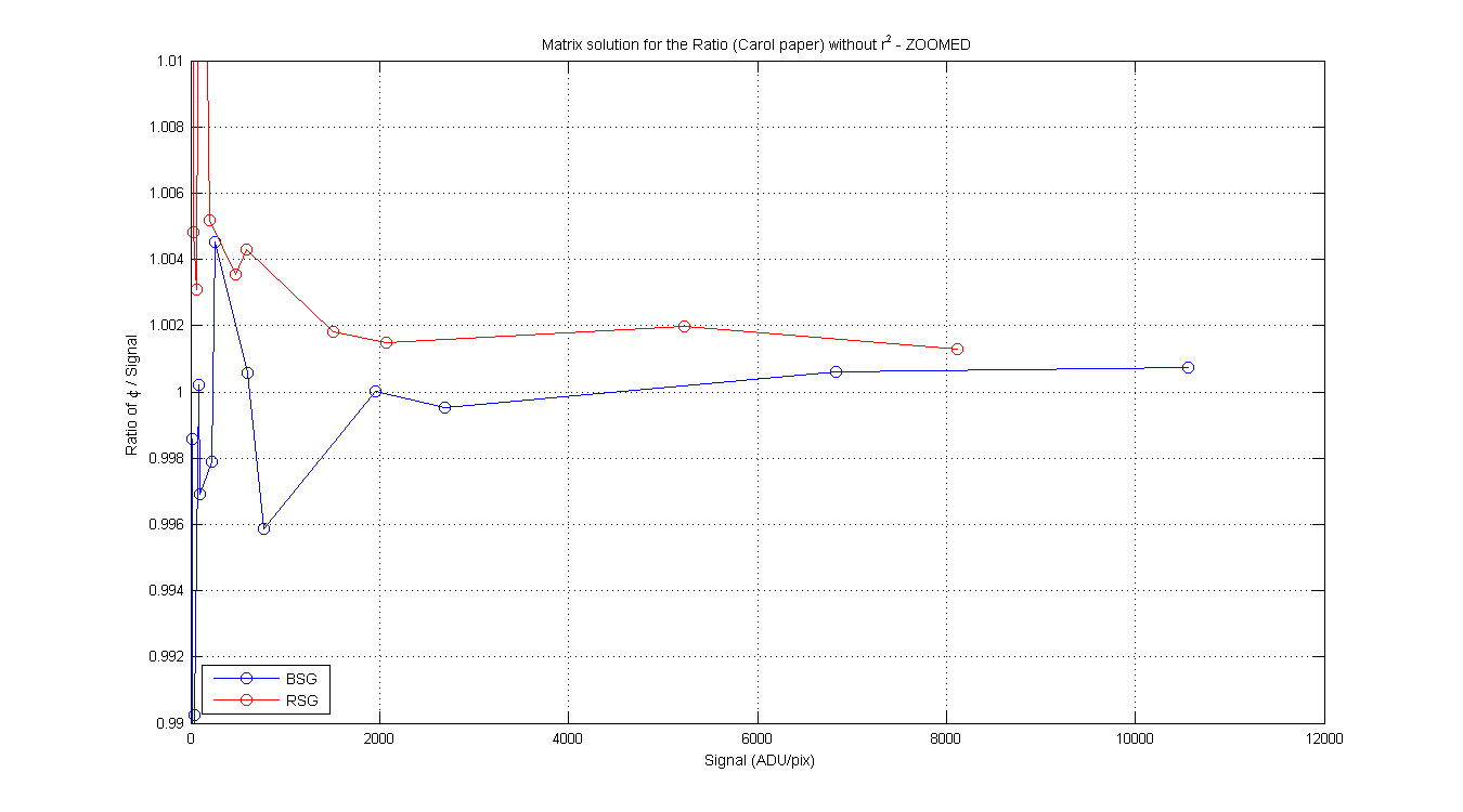
BSG/RSG Table from Carols write-up page 2-3. Column 2 is the RD or S (mean of pixeles around max),
column 3 is the φ from the matrix math, column 4 is the residual from Carols paper and Colum 5 is the
ratio of φ / signal. Same for the RSG. Each of the columns contains the φ, Residual and ratio with and without the r² in the equations.
r coefficents with r²
BSG r values = [ -2.6428 1.5649e-007 ]
RSG r values = [ -0.46338 3.0444e-007 ]
r coefficents without r²
BSG r values = [ 0.21073 ]
RSG r values = [ 2.8223 ]
| BSG |
RSG |
| Aperature |
RD or S |
φ (w r² / wo r²) |
Residual-Y (w r² / wo r²) |
Ratio (w r² / wo r²) |
Aperature |
RD or S |
φ (w r² / wo r²) |
Residual-Y (w r² / wo r²) |
Ratio (w r² / wo r²) |
| A |
18.198 |
16.107/ 18.172 |
0.552/ -0.237 |
0.885/ 0.999 |
A |
13.471 |
11.952/ 14.330 |
-1.055/ -1.963 |
0.887/ 1.064 |
| IA |
25.862 |
|
-0.552/ 0.237 |
|
IA |
18.408 |
|
1.055/ 1.963 |
|
| I |
10.401 |
6.559/ 8.137 |
-1.199/ -2.475 |
0.631/ 0.782 |
I |
7.380 |
7.047/ 8.864 |
0.131/ -1.339 |
0.955/ 1.201 |
| IB |
38.552 |
|
1.751/ 2.239 |
|
IB |
35.982 |
|
-1.187/ -0.625 |
|
| B |
35.433 |
31.101/ 32.865 |
-1.689/ -2.779 |
0.878/ 0.928 |
B |
27.234 |
27.285/ 29.316 |
0.514/ -0.740 |
1.002/ 1.076 |
| JB |
68.227 |
|
-0.064/ 0.540 |
|
JB |
53.095 |
|
0.670/ 1.365 |
|
| J |
36.468 |
34.420/ 36.113 |
0.595/ -0.566 |
0.944/ 0.990 |
J |
27.831 |
26.017/ 27.966 |
-1.351/ -2.688 |
0.935/ 1.005 |
| JC |
120.728 |
|
-0.537/ 0.026 |
|
JC |
92.200 |
|
0.674/ 1.323 |
|
| C |
84.834 |
83.130/ 84.853 |
0.937/ -0.192 |
0.980/ 1.000 |
C |
68.168 |
66.396/ 68.380 |
-1.310/ -2.611 |
0.974/ 1.003 |
| KC |
183.640 |
|
-0.417/ 0.166 |
|
KC |
142.607 |
|
0.616/ 1.288 |
|
| K |
99.472 |
97.455/ 99.164 |
0.624/ -0.519 |
0.980/ 0.997 |
K |
77.432 |
76.370/ 78.338 |
-0.600/ -1.917 |
0.986/ 1.012 |
| KD |
322.625 |
|
-0.253/ 0.353 |
|
KD |
252.982 |
|
-0.071/ 0.629 |
|
| D |
224.501 |
222.290/ 224.024 |
0.424/ -0.687 |
0.990/ 0.998 |
D |
176.293 |
176.097/ 178.095 |
0.258/ -1.020 |
0.999/ 1.010 |
| LD |
479.711 |
|
-0.291/ 0.335 |
|
LD |
374.793 |
|
-0.331/ 0.392 |
|
| L |
255.078 |
254.523/ 256.232 |
2.078/ 0.943 |
0.998/ 1.005 |
L |
198.883 |
197.945/ 199.913 |
-0.487/ -1.793 |
0.995/ 1.005 |
| LE |
862.354 |
|
-2.112/ -1.278 |
|
LE |
668.435 |
|
0.436/ 1.401 |
|
| E |
604.707 |
603.193/ 605.056 |
1.071/ 0.138 |
0.997/ 1.001 |
E |
471.080 |
470.599/ 472.745 |
-0.085/ -1.157 |
0.999/ 1.004 |
| ME |
1370.766 |
|
0.105/ 1.140 |
|
ME |
1069.223 |
|
-1.454/ -0.244 |
|
| M |
770.256 |
765.329/ 767.061 |
-2.376/ -3.405 |
0.994/ 0.996 |
M |
596.499 |
597.054/ 599.055 |
0.910/ -0.266 |
1.001/ 1.004 |
| MF |
2723.117 |
|
-0.824/ 2.265 |
|
MF |
2105.029 |
|
-3.067/ 0.511 |
|
| F |
1958.507 |
1955.481/1958.532 |
-0.984/ -0.187 |
0.998/ 1.000 |
F |
1506.560 |
1505.794/1509.307 |
-0.993/ -0.075 |
0.999/ 1.002 |
| NF |
4652.353 |
|
-8.488/ -2.078 |
|
NF |
3584.916 |
|
-7.845/ -0.435 |
|
| N |
2693.269 |
2689.127/2691.953 |
-2.635/ -1.527 |
0.998/ 1.000 |
N |
2074.942 |
2074.725/2077.996 |
-1.064/ 0.232 |
1.000/ 1.001 |
| NG |
9521.476 |
|
-26.295/ 3.605 |
|
NG |
7314.332 |
|
-34.113/ 0.204 |
|
| G |
6829.184 |
6817.598/6833.339 |
-16.241/ 3.944 |
0.998/ 1.001 |
G |
5228.973 |
5221.318/5239.362 |
-15.516/ 7.567 |
0.999/ 1.002 |
| OG |
17407.813 |
|
-95.275/ -7.549 |
|
OG |
13377.190 |
|
-108.554/ -7.770 |
|
| O |
10559.376 |
10539.718/10567.136 |
-34.463/ 7.549 |
0.998/ 1.001 |
O |
8122.288 |
8101.335/8132.881 |
-40.574/ 7.770 |
0.997/ 1.001 |
Figure 1
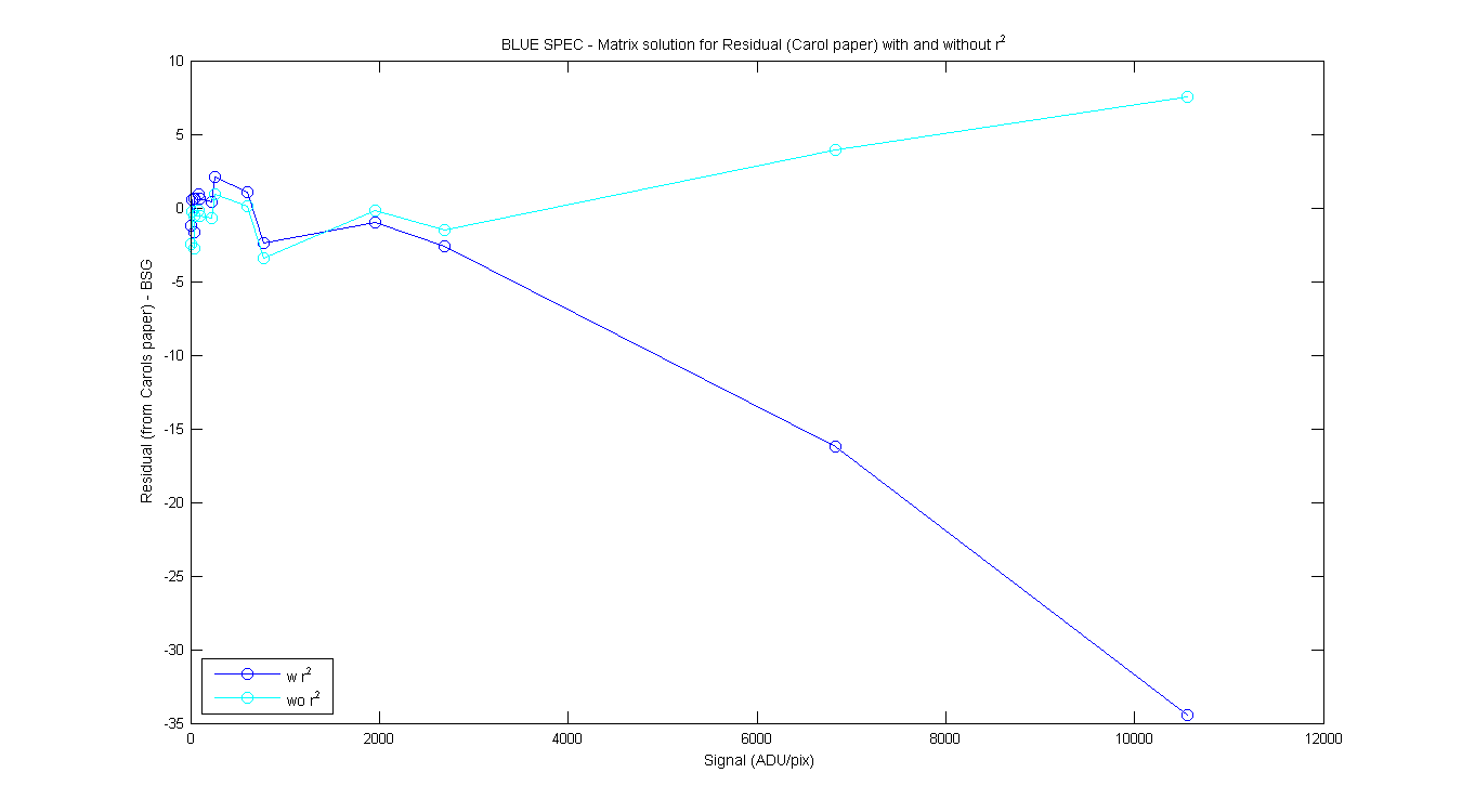
Figure 2
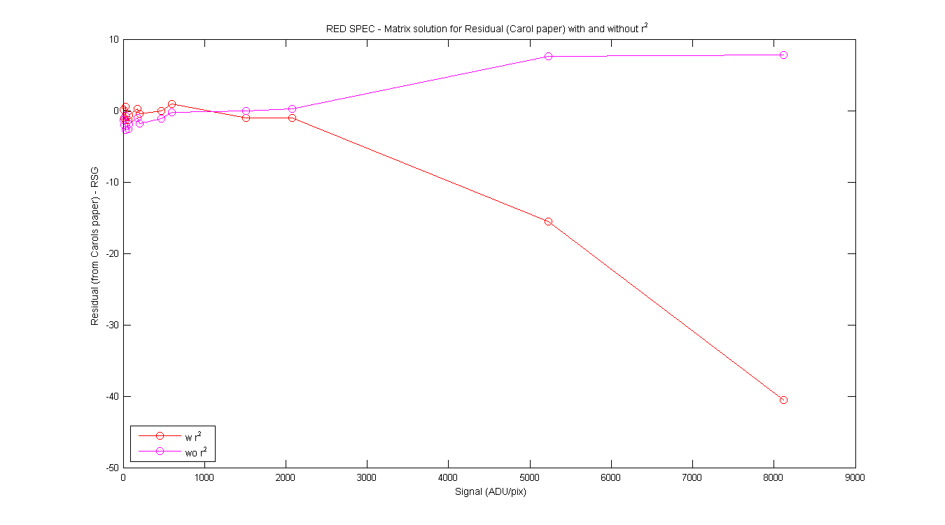
Figure 3
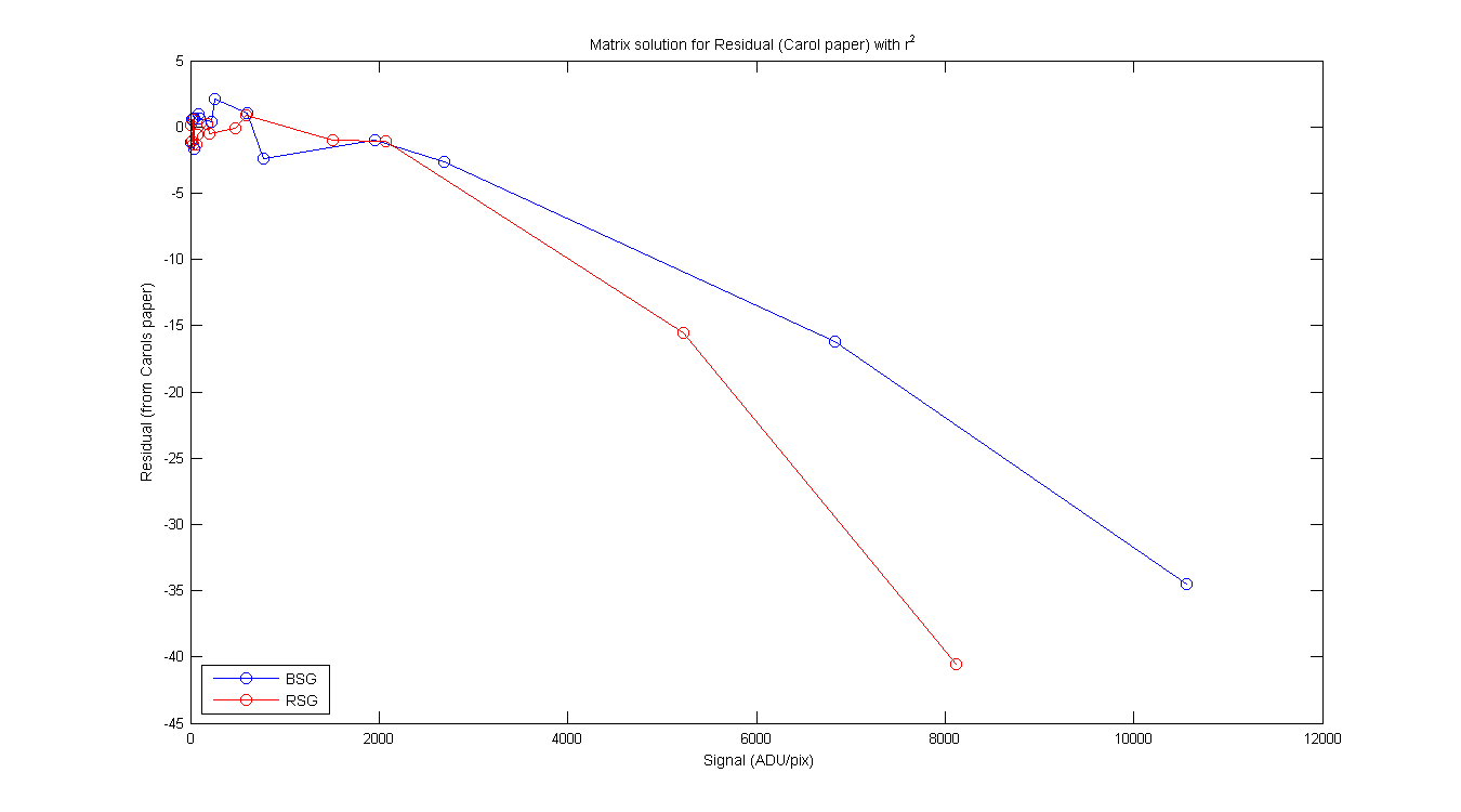
Figure 4
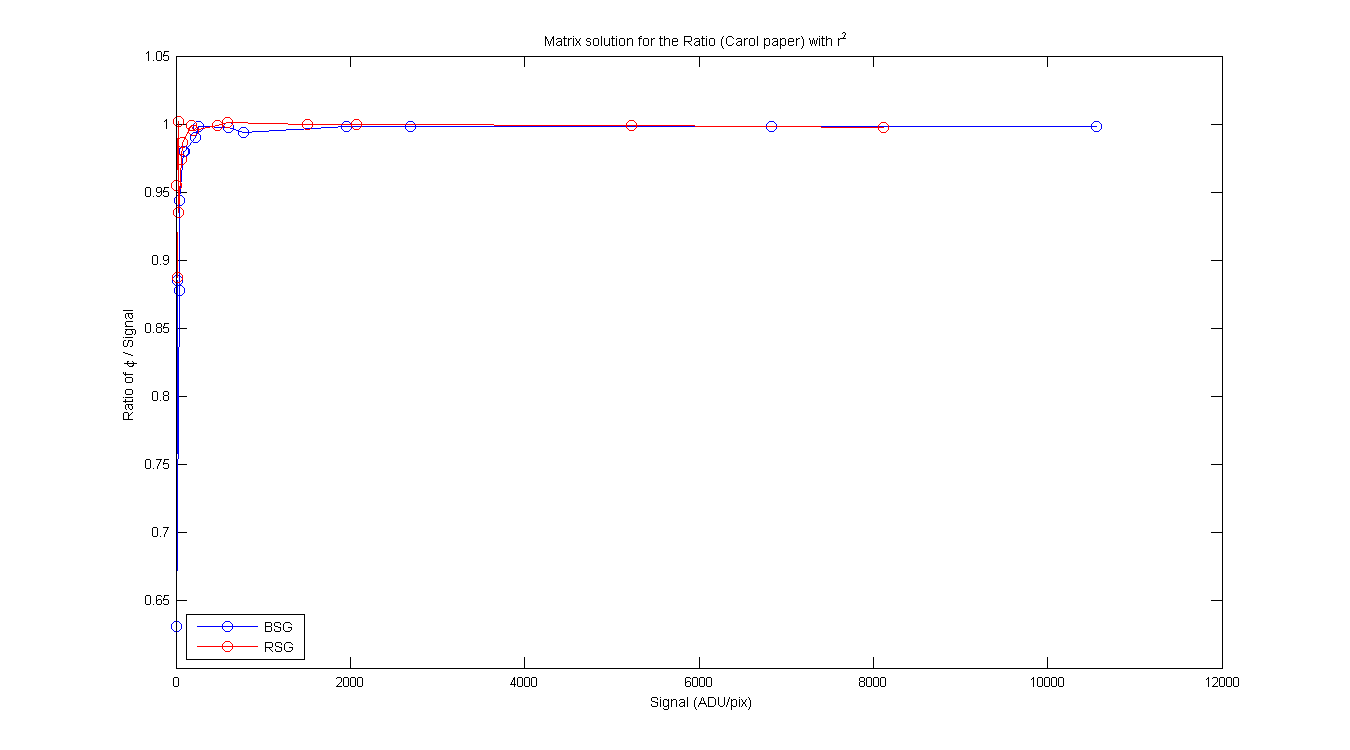
Figure 5
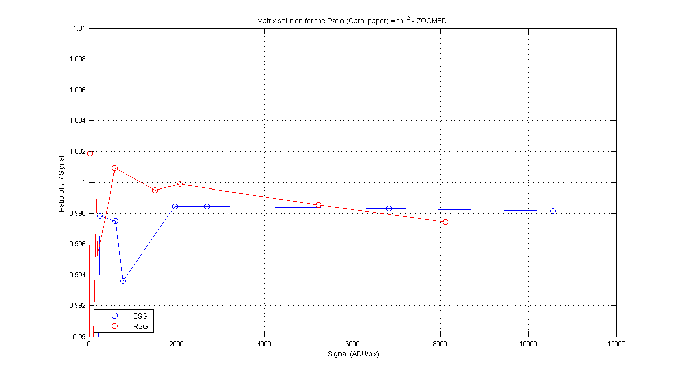
Figure 6
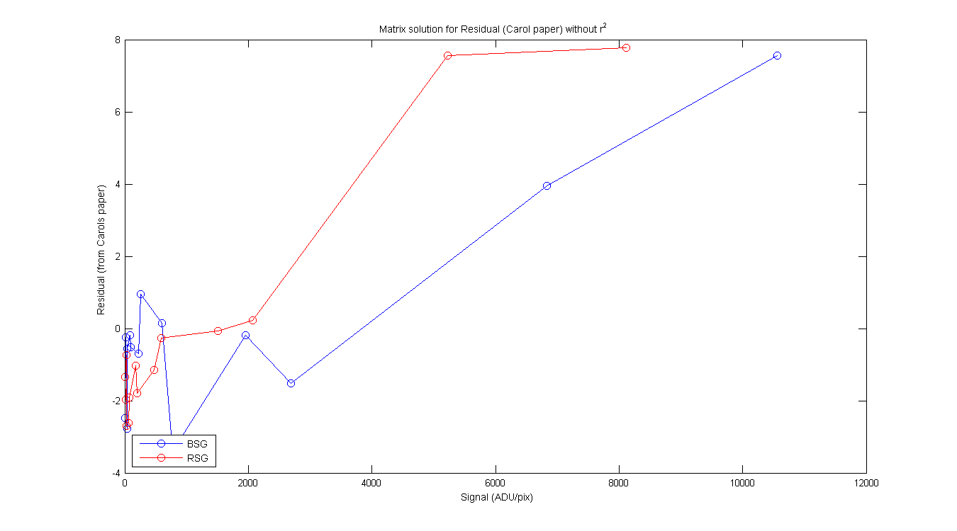
Figure 7
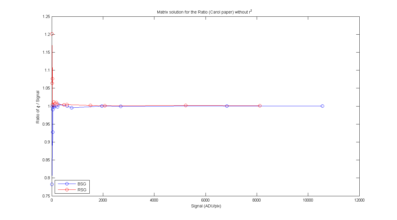
Figure 8
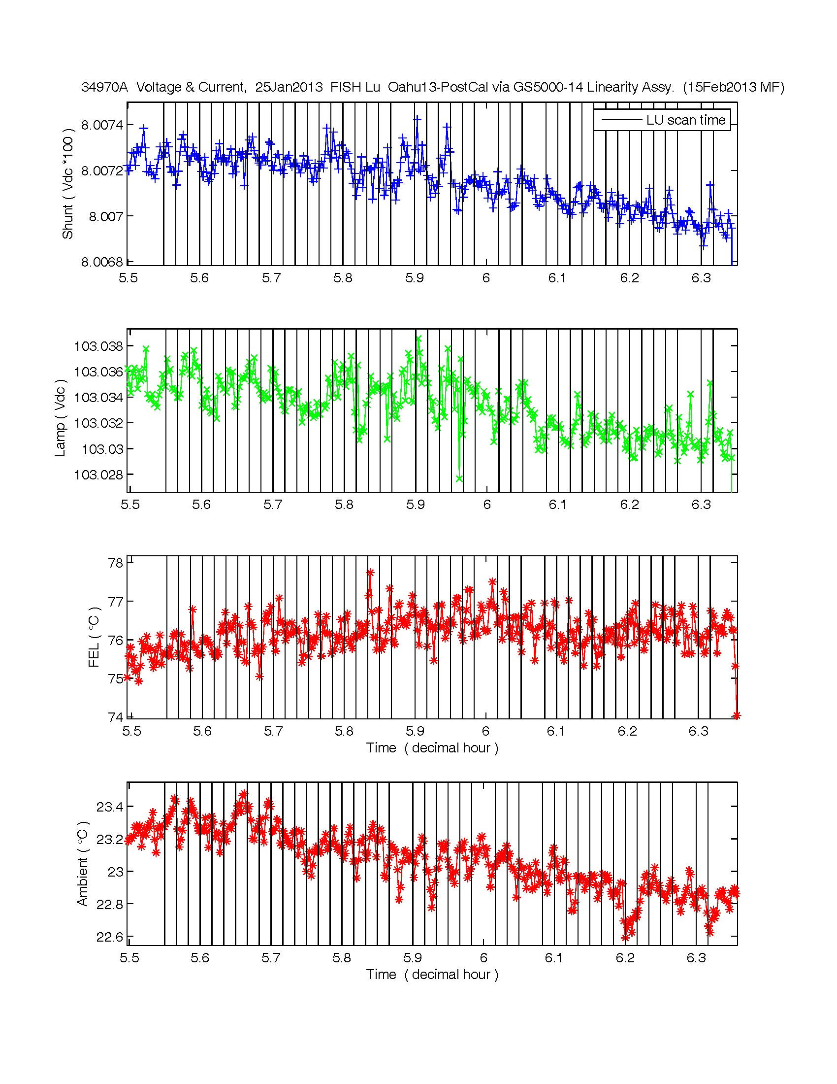
Mike plots of Lamp Voltages and temperatures during the FISH Es linearity experiment #1
pwd: G:\zflora\mldata\MOBY2\20120903_shadowing\Resonon\20121208_linearity
Date: 26-Feb-2013 15:14:29
Created from plt_linearity3_(1)