MOBY262

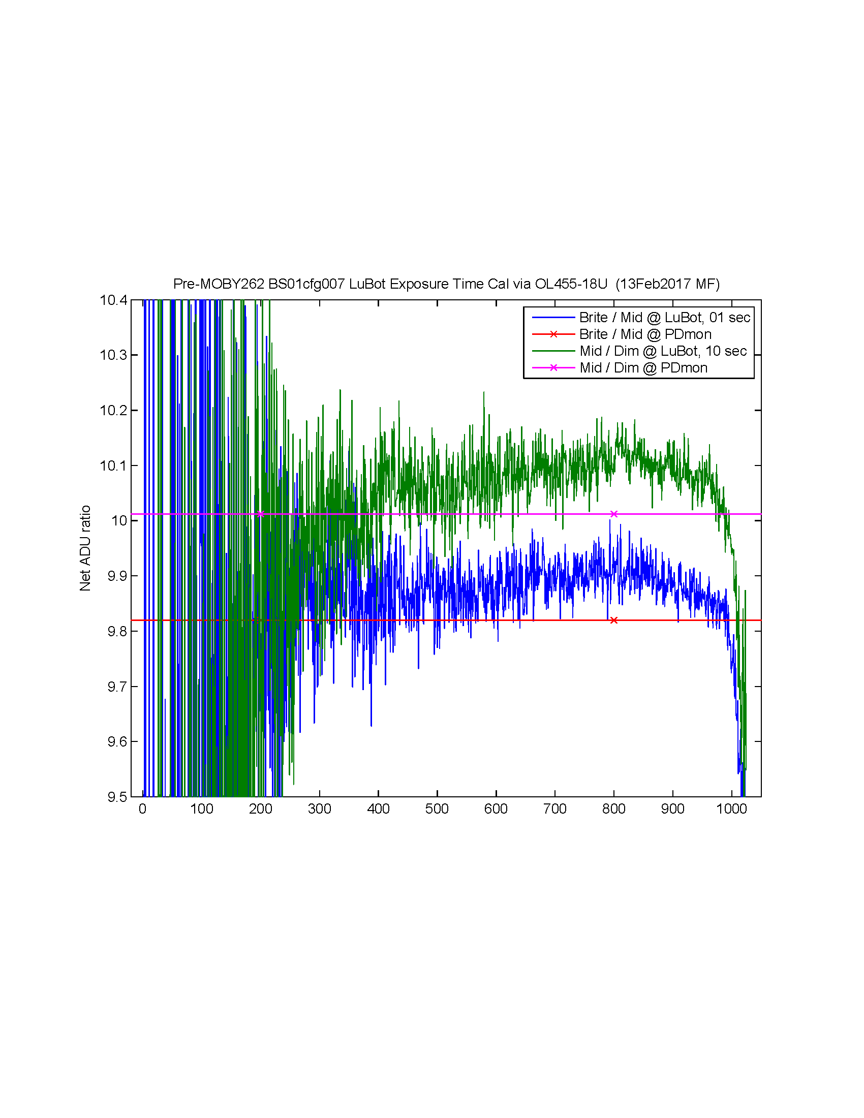
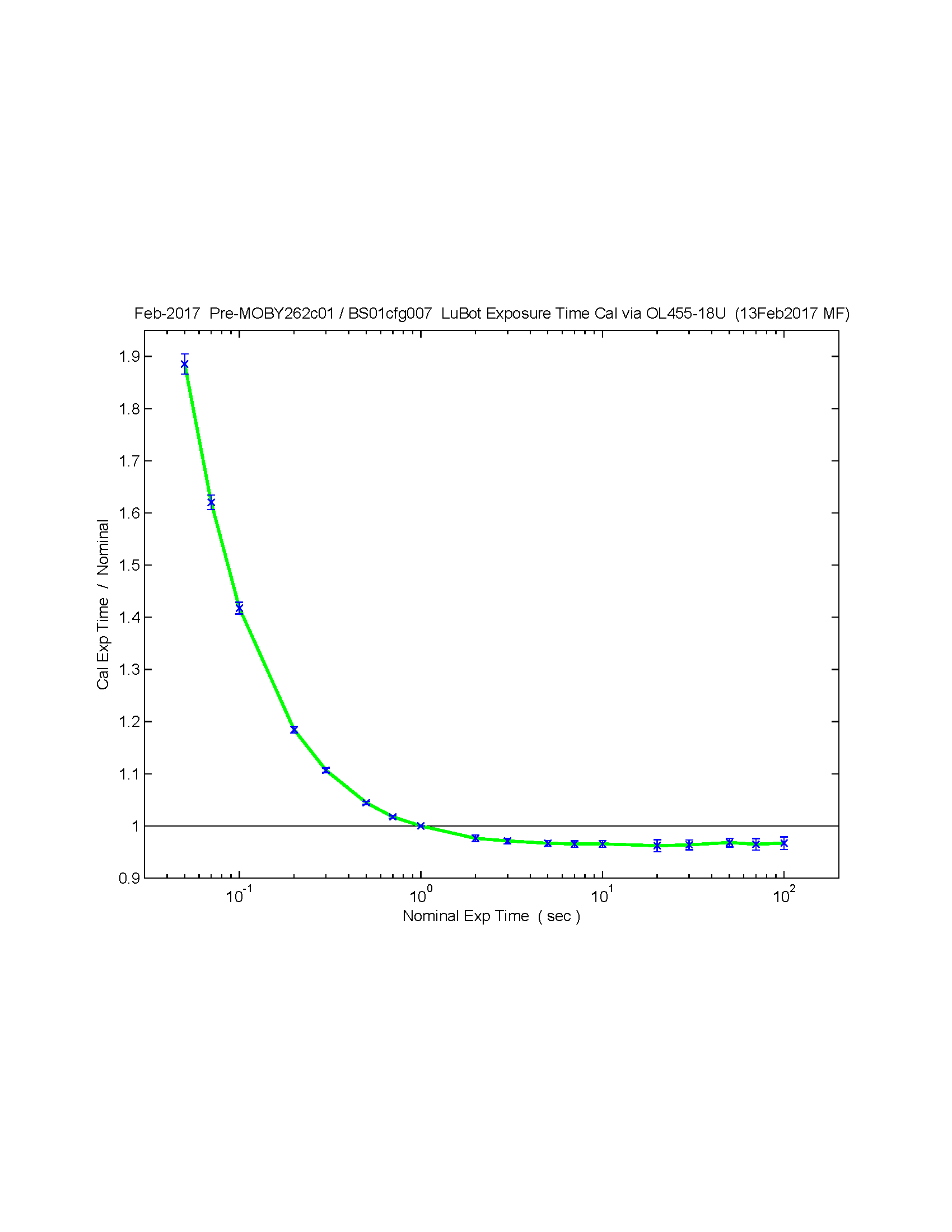
Hi Steph,
I looked at my processing for the last 2 times doing Int Time Cals for pre & post M260 LuBot,
and, I'm not so sure that my approach is an optimum approach,
so you might want to look at what I have to say below and try to improve upon it!

First, "let it be know that" I collected BS data at 3x OL455 sphere settings,
which I call "Brite", "Mid", and "Dim". The shortest exp times were via Brite lamp,
and longest exp times were at Dim lamp.

Second, it wanted to see if what I was aboot to tell you worked, so I ran it through myself.
I processed the Net Signal = Sig minus Bac, in ADU,
using the mean for LuBot Trk#13 = pix 893:936 (your webpage H17-01, page 2.02 "finding tracks").
I used file s,b2017021226...52.fits, which gave 27x net's.

Here is my .m scan-navigation cheat-sheet: (this lines up better in MATLAB editor...)

% scn 1   2   3   4 5 6   7 8 9 10 11 12 13 14 15 16 17 18 19 20 21 22 23 24 25 26 27
% sec 1 .05 .07 .1 .2 1 .3 .5 .7 1   1 2 3 1   5 7 1 10 10 20 30 10 50 10 70 10 100
% BMD B   B   B   B B B   B B B B   M M M M   M M M M D D D D   D D D D D
% 1sec *                 *           *   *        * *

Here is my loader for the PD monitor data:

% OL455 PD monitor (Amps)
%-------------------------
%     1     2     3     4     5     6     7     8     9     10
pd=([.8521 .8524 .8521 .8522 .8524 .8522 .8522 .8523 .8521 .8522]+1)*1e-6 , whos pd % [1x10]
%         11    12    13    14    15    16    17    18
pd=[pd ([.8862 .8857 .8856 .8856 .8853 .8853 .8851 .8852]+1) *1e-7 ], whos pd % [1x18]
%         19    20    21    22    23    24    25    26    27
pd=[pd ([.8829 .8828 .8828 .8825 .8822 .8822 .8823 .8823 .8823]+1) *1e-8 ], whos pd % [1x27]

NOTE: I did not end up using the PD data, but I think the processing could be done
to make use of these, because the transitions from Brite to Mid, and Mid to Dim
agree well between the BS Net Sig ratios and the PD mon ratios
<attached: rb62bs01_exp_1.png>

I checked the Net Sig repeats at 1 sec for the Brite lamp (+/- 0.5%),
and at 1 sec for the Mid lamp (+/- 1%),
and at 10 sec for the Dim lamp (+/- 1.5%).
Since they seemed OK, and the PD mon repeats were essentially 1,
I did my Net Sig "normalizing" to the nearest-in-time
1 sec exposure Net Sig at Brite & Mid lamp settings,
and to the nearest-in-time 10 sec net at Dim lamp setting
(hopefully this will make sense below!).

Here is what I used for Nominal Exposure Time:

% N      1   2 3 4 5 6 7   8   9 10 11 12 13 14 15 16 17 18
nom = [.05 .07 .1 .2 .3 .5 .7   1   2 3 5 7 10 20 30 50 70 100], whos nom % [1x18]
% scn=[ 2   3 4 5 7 8 9 10 12 13 15 16 18 20 21 23 25 27 ];

So, there will be 18x "Calibrated" exposure times for these 18x nominal times.
I get Calibrated times as "rel", by normalizing to 1 sec net signal:

% Brite
rel(:,01)=net(:,02) ./ net(:,01); % #02= 0.05 / 1 sec
rel(:,02)=net(:,03) ./ net(:,01); % 03= 0.07
rel(:,03)=net(:,04) ./ net(:,06); % 04= 0.1
rel(:,04)=net(:,05) ./ net(:,06); % 05= 0.2
rel(:,05)=net(:,07) ./ net(:,06); % 07= 0.3
rel(:,06)=net(:,08) ./ net(:,06); % 08= 0.5
rel(:,07)=net(:,09) ./ net(:,10); % 09= 0.7
rel(:,08)=net(:,10) ./ net(:,10); % 10= 1
%
% Mid
rel(:,09)=net(:,12) ./ net(:,11); % #12= 2 / 1 sec
rel(:,10)=net(:,13) ./ net(:,14); % 13= 3
rel(:,11)=net(:,15) ./ net(:,14); % 15= 5
rel(:,12)=net(:,16) ./ net(:,17); % 16= 7
rel(:,13)=net(:,18) ./ net(:,17); % 18= 10
%
% Dim                                Mid,10sec    Mid,1sec
rel(:,14)=net(:,20) ./ net(:,19) .* (net(:,18) ./ net(:,17)); % #20= 20 / 10
rel(:,15)=net(:,21) ./ net(:,22) .* (net(:,18) ./ net(:,17)); % #21= 30
rel(:,16)=net(:,23) ./ net(:,24) .* (net(:,18) ./ net(:,17)); % #23= 50
rel(:,17)=net(:,25) ./ net(:,26) .* (net(:,18) ./ net(:,17)); % #25= 70
rel(:,18)=net(:,27) ./ net(:,26) .* (net(:,18) ./ net(:,17)); % #27= 100

For the Dim scans, "one can see that" (I hate when they say that!)
I added a correction to get from 10 sec at Mid to 1 sec at Mid (net#18/net#17) -
this is where I think there might be a better way of doing this -
maybe by using the PD monitor to correct between the Brite & Mid & Dim settings ?

Plotting the "rel" net signals on a semilogy it looked like pix 300:900
was a stable range, so I got the mean and std over pix 300:900:

N=[300:900]; nanmean(N),clear ans % 600
for i=1:size(rel,2)
int(i)=nanmean(rel(N,i)); std(i)=nanstd(rel(N,i));
end, clear i, whos int* std* % [1x18]

[[1:18]; nom; int; std./int*100]'
% N    nom      avg        %std
% --    ----    --------   -------
% 1      0.05   0.094278 1.0278
% 2      0.07   0.11343   0.85473
% 3      0.1    0.14175   0.78595
% 4      0.2    0.23689   0.53124
% 5      0.3    0.33199   0.37709
% 6      0.5    0.52217   0.29506
% 7      0.7    0.71216   0.23327
% 8      1      1         0
% 9      2      1.9524    0.63782
% 10      3      2.9134    0.55747
% 11      5      4.8333    0.55972
% 12      7      6.7566    0.62245
% 13     10      9.6539    0.66262
% 14     20     19.24      1.1847
% 15     30     28.909     0.97703
% 16     50     48.403     0.85737
% 17     70     67.533     1.1422
% 18    100     96.7       1.2415

Which plotted up like this:
<attached: rb62bs01_exp_2.png>

I do NOT think this std is a valid uncertainty estimate,
because it does not include the unc for the transition
between 10 sec to 1 sec at Mid lamp setting...

Here are my results:
<attached: BS01_exptimecal(rev13Feb2017).txt>

I think we can use this to get started, and worry aboot improving
upon this approach when we have some more time...
MF

All the raw data files and their images , Table of KEYWORDS variable
Page Number	Link	Description	Date
1.01	Day 01 - 6 Feb Raw Data , Table	DAY01 - Oriel, 4x iris @ shutter block adjustment for Tracks 1,9 11 and 13 - cfg006	Feb 6, 2016
1.02	Day 02 - 8 Feb Raw Data , Table	DAY02 - Oriel, 4x iris @ shutter block confirming adjustment for Tracks 1,9 11 and 13 (after Mark secured iris settings) - cfg007	Feb 9, 2016
1.03	Day 03 - 10 Feb Raw Data , Table	DAY03 - OL425 lamp data of LuTop, Mid and Bot with heads, shutters and iris - cfg007	Feb 10, 2016
1.04	Day 04 - 11 Feb Raw Data , Table	DAY04 - Lamp cals of Es, LuTop, Mid and Bot with heads, shutters and iris - cfg007	Feb 10, 2016

Day01 - Oriel, 4x iris @ shutter block adjustment for Tracks 1,9 11 and 13 - cfg006
2.01	iris block	Confirming Mikes Iris Block numbers	Feb 8, 2017
2.02	finding tracks	Looking at track definitions	Feb 8, 2017
2.03	Saddle shape changes	Changes to saddle shape with iris addition	Feb 8, 2017
Day02- Oriel, 4x iris @ shutter block confirming adjustment for Tracks 1,9 11 and 13 (after Mark secured iris settings) - cfg007
3.01	iris block check	Confirming Mikes Iris Block numbers after Mark secured iris settings	Feb 9, 2017
Day03 - OL425 lamp data of LuTop, Mid and Bot with heads, shutters and iris - cfg007
4.01	rough rsp	A rough intial system response of the BS01 with iris, shutters and Lu heads	Feb 10, 2017
Day04 - Lamp cals of Es, LuTop, Mid and Bot with heads, shutters and iris - cfg007
5.01	Es rsp	Es rsp before the disconnected end-block	Feb 11, 2017
5.02	Es rsp repeatability	Es rsp before and after the disconnected end-block	Feb 11, 2017
5.03	Lu rsp	Lu rsp	Feb 11, 2017
5.04	int time cal	My intial look at Mike int cal data	Feb 11, 2017
5.05	%std Es and Lu	Looking the %std of Es repeatability for Es and Lu net signals	Feb 13, 2017
5.06	Ghosting check	Checking to see if light from track 1 is showing up on track 14 in the UV	19 Jan 2018

Hawaii-2017-01 experiment with new MOBYrefresh blue Resonon - BS01cfg006 and 007