Hi Steph,

If you are up to it, there are some BS02cfg01 data in ftp1/Mike/HI-2016-01/

I just ran the Oriel incandescent lamp with all 14 FOs at the exit port of the 12" Spectralon sphere. The alignment was VERY rough!  See the photos.

I took 5x backgrounds with the sphere lamp light off, then I took 5x ambients = sphere light off, then I took 5x signals = sphere light on.

Then I found FO# 8 and coupled it alone to the sphere.  See photos. I took 5x signals = sphere light on, then I took 1x ambient = sphere light off, then I took 1x background

All data were collected at 0.5 sec exposure, 4x gain, speeds= 4.25 usec Vert, 3 MHz @ 16 bit Horiz, 35/35 ms shutter delays, CCD was -40 degC.

I think I messed up the exposure time setting though, because at the end it looked like the max sig was ~1.5e4 ADU, but the readout plot was showing 4e4 ADU when I was scanning (?) - I am still having trouble running the SOLIS software...

There were no Aux data collected. Now I'm going to try to run thru a set of laser lines with FO# 8 only.

Good Luck, MF

-------------------------------------------------------------

Hi Steph,
I just scanned 11 laser lines, at 300 : 50 : 800 nm,
for at total of 22 files = sig & bac,
all with FO# 8 only.
There is a pg. 2 of 2 log sheet for this.
There are no more photos.
That's it for today/tonight.
Luck, MF

Hi Steph,
I had to change the name on the aux file from yesterday - it was missing a zero at/near the end.

Tonight I started by re-running the same same scans as last night = only T7 open, with same exposure times, 1.5 thru 0.035 sec, to see if this is repeatable.

Then I did the same exp times with all tracks illuminated. To see if the number of tracks illuminated affects the exp time cal.

Then I continued with all tracks on, for longer exp times, which meant stepping down the lamp voltage twice. When I had to change the lamp voltage I scanned sig & bac at both the high & low lamp voltages, keeping the exp time same, so we can calculate a spectral ratio to "adjust" the lamp spectra from high to low across the lamp voltage change.

I think you might have run through this game before yes? If this makes no sense let me know!

FileZilla & the www are complete junk tonight!  <100 kB/s, >10 crashes...

I think I may have sent you a version of this aux doc yesterday that was missing the end of pg. 1 descrip of the time stamp?
<attached: Aux_data_via_LabJack_for_MOBY-Refresh(rev1).pdf>

MF

Hi Steph,
The HTM2500LF was used as the external/ambient %RH  & degC with the FISH = 1 with Blue & 1 red Red, inside the big black box house for both instruments.

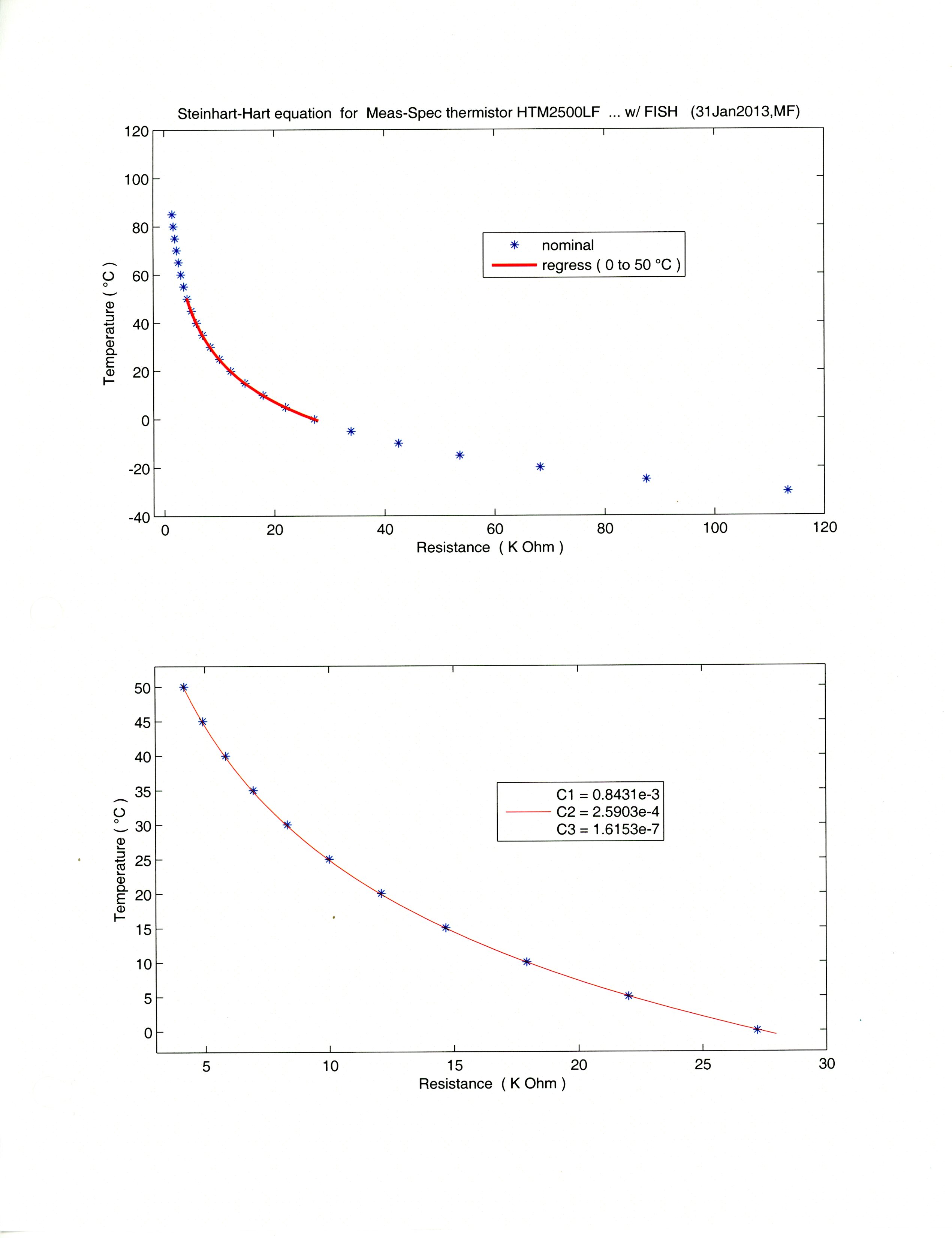
Attached here is the manual <HTM25X0LF(revC).pdf>, where pg.4 bottom equation is how to get %RH, with temperature compensation, and my notes for pg.6 of same manual <%RH_&_NTCthermistor_06.png> which shows the eqn you need to convert thermistor Ohms to K & degC, and my Steinhart-Hart regression coefficients for Ohms to degC<HTM2500LF_Steinhart-Hart.jpg> = coef's on pg.6 notes.

I'm going to try to dig up my MATLAB code for FISH aux, because it seems to me there should be a Vin somewhere in the %RH eqn - i.e. should Vout be a function of Vin ? Maybe not, because manual pg.2 says Supply Voltage = 4.75 to 5.25 Vdc...

One (more) detail I forgot to note: for HI-2016-01 ambient the HTM2500LF S/N = 122702-37. Which I don't think really matters much, but I'll add that to the pdf writeup.

If I have time I'll try to add all the conversion equations & coefficients to the pdf!
MF

I kinda knew this, but here are the spectral ratios for the 2x lamp Voltage changes ... which are not very flat ...
<attached: C:\data\2016\HI-2016-01\BS02cal\plots>

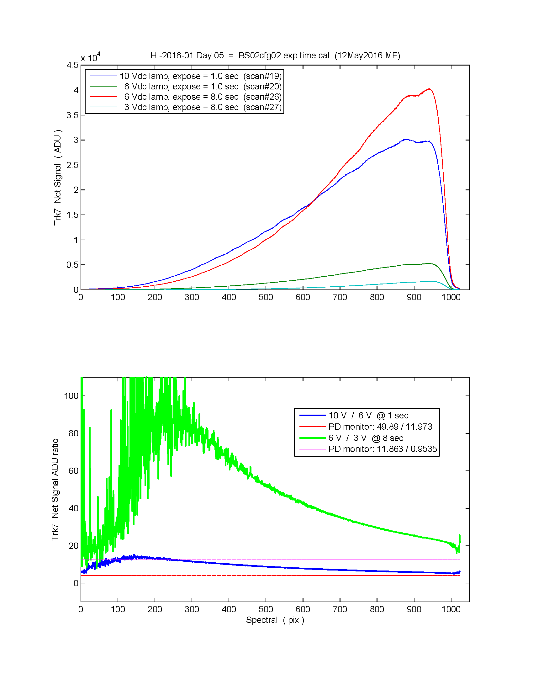
THat PLot I SEnt YEsterday, with the day5 10V/6V & 6V/3V spectral ratios was not correct.
It turns out one needs to ratio Net Signal (my yesterday plot ratioed Signals).
Here is the Net Signal ratio plot ... with the PD monitor ratios overplotted ...
<attached: HI-2016-01_day5_MF.png>

Hi Steph,
FileZilla is running 3x faster tonight, only 2x crashes so far...

I added an iris between the lamp and the sphere today, so we shall see if the 2x step-downs in output level are more spectrally flat than last night...

And, I used a different input port on the integrating sphere for the Oriel incandescent lamp + iris.  This port has a small internal baffle.  This port was meant to be an input port for a fiber optic.  So there is the chance that the output port uniformity might be better (?).

Otherwise, I repeated the all-track data from last night: 1x aux file, 2x log sheets, 26x sig&bac scans, 2x amb scans. I also took 3x photos of the Oriel lamp setup.
MF

Thank you!  I am going to have to think aboot this some...  MF

P.S.  here is the aux doc updated w/ HTM S/N & "Ambient" naming.
<attached: Aux_data_via_LabJack_for_MOBY-Refresh(rev2).pdf>

Hi Steph,
THat PLot I SEnt YEsterday, with the day5 10V/6V & 6V/3V spectral ratios was not correct. It turns out one needs to ratio Net Signal (my yesterday plot ratioed Signals). Here is the Net Signal ratio plot ... with the PD monitor ratios overplotted ...<attached: HI-2016-01_day5_MF.png>

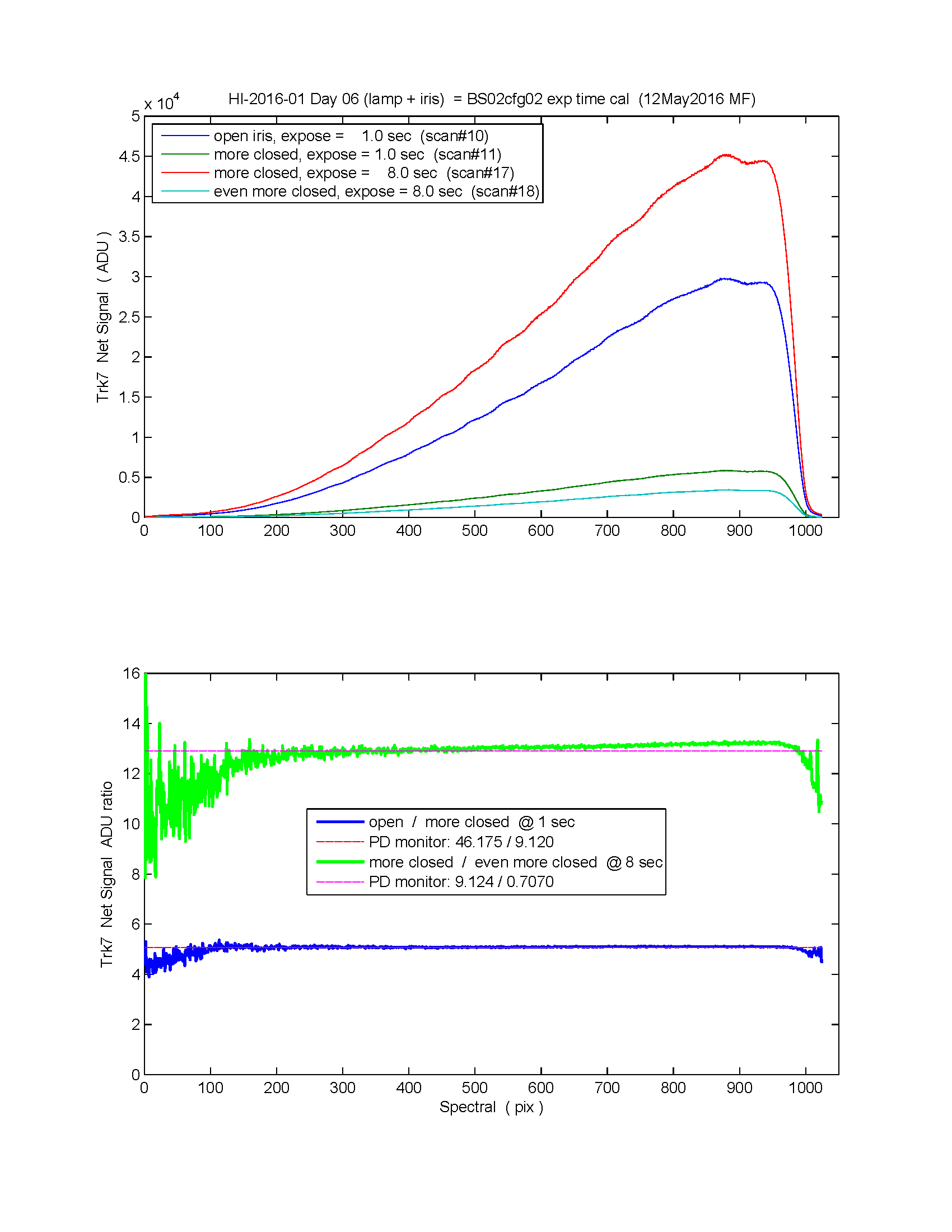
And here is same for day6 via iris changes to dim the sphere output <attached: HI-2016-01_day6_MF.png>

For Day6, it would seem that we could be averaging spectral pixels ~300:900 to get an estimate of the Net Signal change to compare with the exposure time change.

Now I will look at your day6 plots!
MF

Hi Steph,

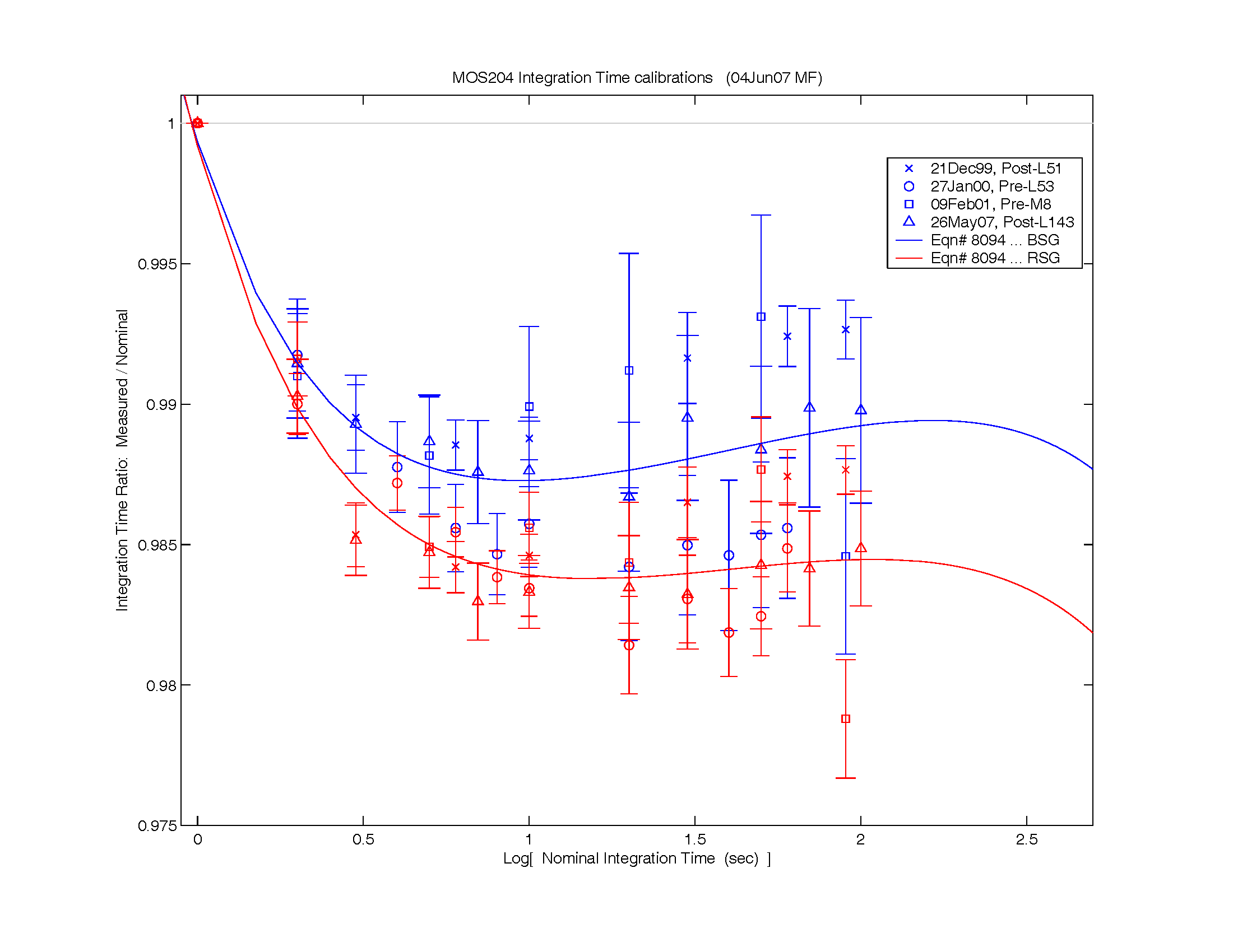
I think it might be wise to re-run day6 with only 1-trk illuminated, because there looks like some trk-to-trk diff at short exp times... This is where errorbars might offer some insight into whether these differences are significant - I'm thinking about this kind of plot <attached: m4int_BvsR_04jun07_3.png> where one can see that each of the 4x int cals for MOS204 had noise, and flyers, then you try to fit a regression line and see if the individual points +- their error are significantly different from the best-fit.  In our case here, we would check
if there is really need a separate exp time cal needed for each track...

I suppose I could also change up the exposure times to fill in gaps some...

And I suppose I could reverse the order and run from low-light/long-exposure through high-light/short-exposure...
Then we can compare day6 T7 bright-to-dim  versus  day7 only-T7 dim-to-bright...

MF

Hello again,
Last email for today - I promise !

Day07 data are heading your way. Same physical setup as Day06. Only Trk7 = open, from dim light to bright light 3x brightness steps via 3x iris settings from 100 sec to 0.035 sec exposure times trying to repeat some from day4,5,6 plus some new ones. 2x log sheets, 1x aux file, 31 sig & bac scans, 62 total files, total size: 130,527,360 bytes.

Smoking fast inter webs tonight! (oops, it just slowed down by 4x...) (and now it did crasht...)


Aloha, MF

Hi Steph,
Sorry this took all day to answer - I had to go back to my MOS204 notes to remember what I had done in the past and I fought with several errors (and there are at least two more errors I found that remain un-fixed right now...).

In that plot I sent of the different fits running through the error bars for MOS204, those fits were via TableCurve 2D - otherwise I do a 5th order regression on log-log data (!)

It looks like this has been my (approximate) int time cal processing approach for MOS2:

1.) get Net Signal ADU from lites & darks
2.) apply MOS2 thermal correction to NetSignal ADU (via TT7 temperatures)

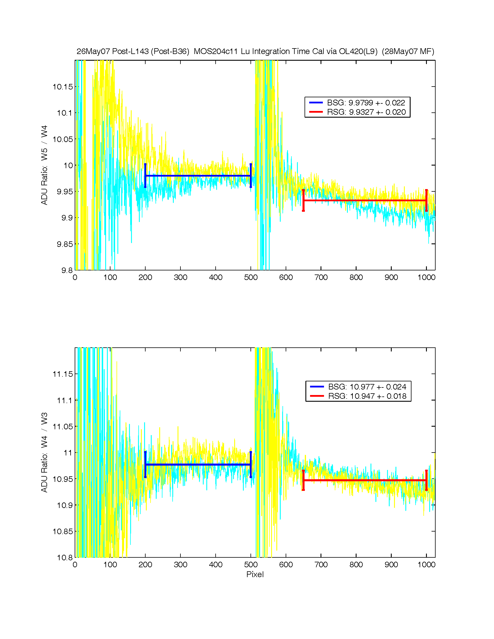
3.) get NetSignal avg & std for BSG pix 200:500, and RSG pix 650:1000 (or other stable pix range)
4.) find the aperture-change lamp-step functions for BSG & RSG
ex. 2007 post-M236 MOS204cfg11 <attached: m4_int_1.png>
5.) compare avg+/-std BSG & RSG step functions vs expected from aperture-wheel-ratios (or monitor ratios)

5.) find spectral NetSignal ADU ratios (1024 pix) relative to 1 sec int time
... some scans will need adjustment via step-function to normalize to 1 sec lamp range ...
... these "adjustments" can be via avg or via full spectral step-functions ...
6.)  get RelativeNetSignal avg & std for BSG pix 200:500, and RSG pix 650:1000

(NOTE: this std does NOT include any uncertainty from the lites & darks (i.e. SNR), but it should !)

7.) plot
> plot([-1.5 2.5],[1 1],'k'),hold on
> errorbar(log10(nomInt), avg_RelNetSigBSG./nomInt, std_RelNetSigBSG./nomInt, 'b')
> errorbar(log10(nomInt), avg_RelNetSigRSG./nomInt ,std_RelNetSigRSG./nomInt, 'r')
> xlabel('LOG10[  nominal int time  ( sec )  ]'), ylabel('cal  /  nominal')

7.1.) compare the BSG & RSG, and typically average together  to have one int time cal for both...
... AVG = avg( avgBSG avgRSG )  &  STD = avg( stdBSG stdRSG )

8.) combine AVG & STD from cal #xx with all previous cals

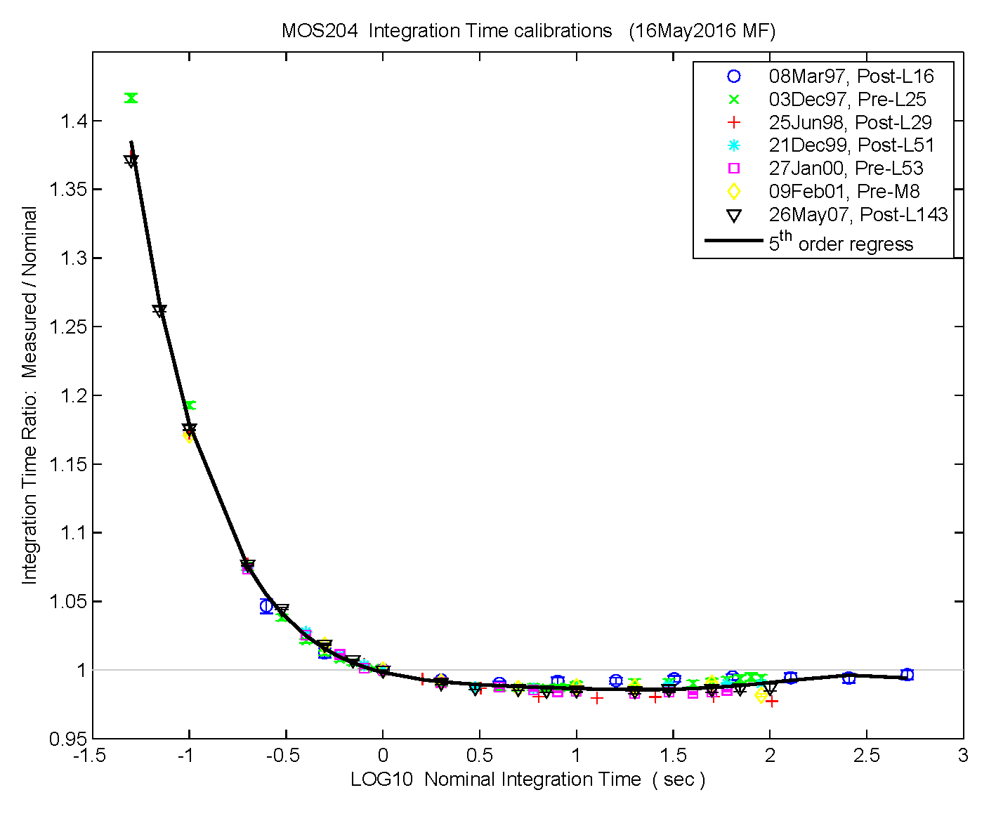
9.) 5th order regression of "log10" data
> xdata = log10( [ cal01_nominalIntTimeSec cal02_nominalIntTimeSec ... calxx_nominalIntTimeSec  ] )
> ydata = log10( [ cal01_AVGRelNetSig           cal02_AVGRelNetSig          ... calxx_AVGRelNetSig            ] )
> myregres % 1=poly, 5=order  ==  Dr. B.'s regress() + my tweaks

ex. MOS204 cal01 ... cal07:
Polynomial Regression: Order =       5
-------------------------------------------
i      B(i)                Sb(i)                 F(i)
0 -7.5234e-004  3.6172e-004  4.3260e+000
1  9.8470e-001  6.5196e-004  2.2812e+006
2  2.3619e-002  1.0620e-003  4.9457e+002
3 -2.1780e-002  4.3328e-004  2.5269e+003
4  9.9042e-003  5.7558e-004  2.9609e+002
5 -1.6044e-003  1.6413e-004  9.5558e+001

r^2                      1.0000
Std Error of Estimate    0.0020
N                           105
Degrees of Freedom           99

10.) overplot 5th order log-log regression  vs  errorbar() for each individual cal
...  ex. <attached: m4int_regress_16May2016.png>

Clear as mud right?
MF

Hi Steph,
I re-ran the exp time game again again tonight, with trk#1 & 14 on. There are 2x log sheets, 1x aux file, and 35x sig & bac scans. I repeated most day7 exp times and tried to fill in a couple holes.

I had a problem when I started log sheet pg.2-of-2, for scan #19 - I got confused with the 0.9 & 0.8 sec scans at the bright-lite setting... I may not have gotten scan #18 at 1 sec ? So at the end I repeated the 1.0 sec scan as scan #35. Sorry for any confusion there...

Aloha, MF

Mike

I have been looking at the data and I think is there is another issue.  I think file 17 was done at the same level as file number 35,  not at the middle level.  When I ratio 17 and 35 to get the step down correction ratio it is 1.  I am going to a thesis defense then I will be back to figure this out. 

Steph

I think you are correct:
scan #17 @ 1.0 sec should have been collected at the mid-level-lamp setting, but it is the same as scan #35 @ 1.0 sec, collected at the high-level lamp setting, and both scans #18,19 were @ 0.9 sec, high-level lamp.

I managed to not collect the cross-step scan at the mid-level lamp. Last night I was afraid I did something like that. Theoretically we could use the PD monitor levels to get the mid-to-bright lamp step-factor...

Maybe suppose I should repeat this again tonight - correctly... I'll probably go from short-exposure / bright-lamp  to  long-exp / dim-lamp so as to not EXACTLY drive myself mad.

Hi Steph,
Tonight, for day09, I repeated last night's day08 data set, with (hopefully) correct exposure timing control = 34x sig & bac scans + 2x log sheets + 1x aux file.
Thanks, MF

Hi Steph,
Looking again at the Habauzit 2003 MOS Bench Unit paper, I was thinking maybe we could try two more things before giving up with present BS02 setup:

Fig.5, Linearity keeping exposure time at 1 sec while varying sphere radiance level to collect images with low counts up to high counts

Fig.6, Exposure Time varying exposure time from low to high seconds while also varying sphere radiance level to keep the number of counts ~constant in order to eliminate possible nonlinear effects

The Habauzit Fig.6 approach should be a sanity check of what we have been doing up to now, which did not keep constant ADU and hence convolved any linearity effect.

Both of these approaches directly rely on the sphere monitor for normalization - but, we do not really know much aboot our sphere monitor, except that much of the previous exp time step-factors seem to agree: change-in-ADU  vs  change-in-PD  (micro Amp DC).

So, I got close last night to writing a logger for the PD monitor (i.e. LabVIEW reader for the Keithley 6517B electrometer), so we will have (another) ASCII timeseries of PD level (something I started thinking aboot in summer 2014).


MF

Hi Steph,
We have more BS data !

I did 2x test scans to check the FITS time stamps "DATE" & "FRAME", by starting a 60 sec and a 1 sec exposure signal scan at precisely know computer times ( i.e. as close as I could get to a *:00 sec & *:30 sec start times ) and, just as you thought, DATE == FRAME == start-of-exposure-time.

I ran the new LabVIEW VI to log PhotoDiode Monitor current, to log filename = pdmon2016052601.txt.  I wrote down approximate PD microAmps as I took scans as a check against what was logging to the file, but my program flashes the Keithley DVM front panel and it is hard to read PD levels.  I ran the logger at 200 msec dT.

I tried to repeat the Trk7 exposure time cal by the Habauzit 2003 method: "The radiance was changed along with the exposure time to keep the number of counts approximately constant in order to eliminate any possible nonlinear effects."  So we should follow their data processing description for Fig.6: "The averaged number of counts, normalized to the monitor signal, was divided by the exposure time. This result was then normalized by the count rate at 1 s to get a value y(t) for each exposure time t."

However, it must be noted that we have no idea how linear is the response of our PD monitor! (PD = Labsphere D8-SI-100-TE + TEC = SphereOptics)

The "approximately constant number of counts" was 40k max, but this was at 1 sec exp time, so there are no times < 1sec. I think this could be remedied by starting with a brighter lamp Voltage, and keeping max signals ~30k ADU...

Good Luck with this one!  MF

Hi Steph,
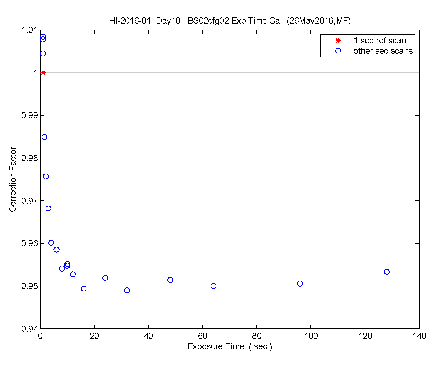
I think I agree with your day10 plot, although I get a slightly different answer <attached: HI-2016-01_day10_MF_1.png>

Here is my modified-Habauzit data processing approach:

The background image was subtracted from signal image, and counts were averaged over spatial pixels 455:503 for Track#7 (ADU/pix).  The spectral net signal counts were divided by the exposure time (ADU/pix/sec), then normalized to the count rate at 1 sec, and averaged over spectral pixels 200:900. This result was then normalized to the monitor signal averaged over the exposure time.

So, from this I now have an avg & std of the PD mon over each exposure time, and, over pix 200:900 I have an avg & std ADU/pix/sec relative to 1 sec, from which I will try tomorrow to to combine uncertainties, from the std's, to put errorbars on the dots...
( I guess I also have a spectral avg & std for the track over the spatial pixels... )

I think the PD mon log file helps!  And the PD levels in the file agree with what I was writing down from the Keithley front panel, so that is encouraging!
MF

Hi Stphaine,
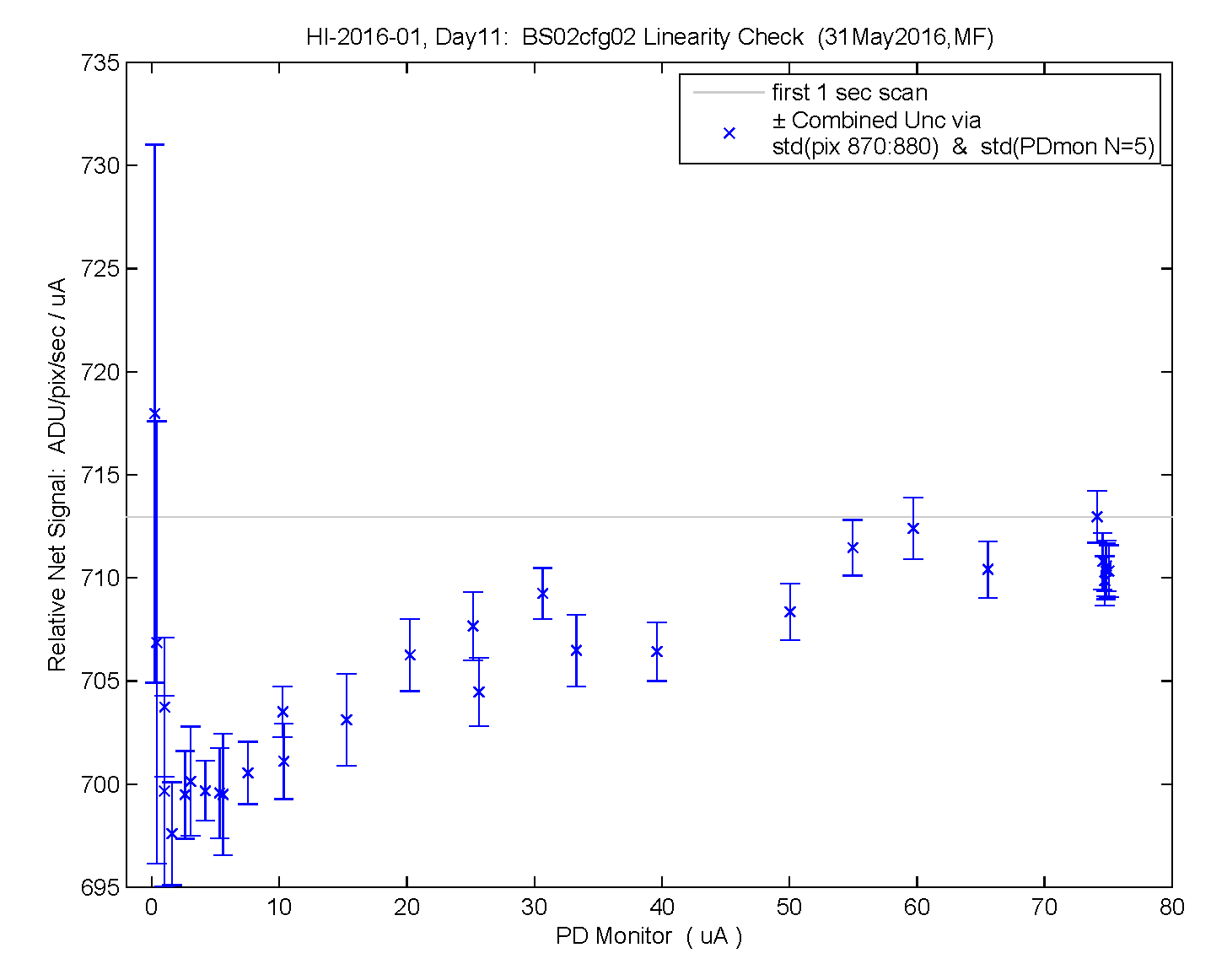
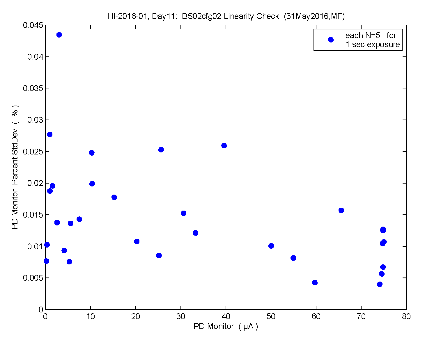
There are Day11 data headed your ftp way:
1x aux file + 1x pdmon file + 2x log sheet scans + 31x sig/bac sets = Habauzit 2003 linearity check, with all scans @ 1 sec exposure time while varying the output of the integrating sphere via open/closing the iris on the Oriel incandescent lamp.

I am not certain if we are checking the linearity of the BS02 or if we are checking the linearity of the PhotoDiode monitor? But it will be interesting to try to reproduce Habauzit Fig.5!

I did 7x repeats at the highest-radiance / open-iris setting over the course of the 31 scan sets.  This should tell us something aboot the stability of this setup - I wish I had done more 1 sec repeats last night for the exposure time check... Looking back at my MOS int time cals, in the more recent ones I started repeating the nominal / 1 sec scans VERY OFTEN to try to remove any time drift of the setup during the run.

Happy LONG weekend, MF

Hi Steph,
Thanks!  I was just trying to figure out how get the Habauzit Fig.5 & Eq.4 uncertainties...
I like that Steve used the Poisson sqrt( N ) estimate for delta Si !

Are your black lines linear fits ? Maybe you could show the a & b coefficients, and the r^2 & SE & N numbers? Another thought I had for a helpful plot would be residuals from a linear fit... I bet they might show some leftover curvature...

One other thing that might clean up the x/y axis a bit is if we show micro Amps instead of Amps for the PD Monitor...  ( or maybe not.. )

MF

Here's an example of what I was thinking r.e. micro Amps - ex. xlabel() which eliminates the 10^-8 exponentiation clutter.<attached: HI-2016-01_day11_MF_1.png> These %Std's for N=5 PD points seem encouraging to me! I was guessing at the 200 msec data logging rate. I think the Keithley could go faster if we need but I I'd need to understand the autoranging which slows it down the way I'm using it now.

I just sent Labsphere an email inquiring aboot the spectral range of said PD...

I'm getting something like this:
<attached: HI-2016-01_day11_MF_2.png>

where the unc is DOMINATED by the std for 11x pix 870:880

i.e. the std for the 5x PD mon Amps are ~10x to 200x less than than the std for the 11x relative net signals in  ADU/pix/sec / A

I will want to check what I am doing here again tomorrow !